|
GraphLab: Distributed Graph-Parallel API
2.1
|
|
GraphLab: Distributed Graph-Parallel API
2.1
|
The Graphical Models toolkit contains a collection of applications for reasoning about structured noisy data. Graphical models provide a compact interpretable representation of complex statistical phenomena by encoding random variables as vertices in a graph and relationships between those variables as edges. Given a graphical model representation, we can then apply Bayes rule to quantitatively infer properties of some variables given observations about others. Graphical models also provide the unique ability to quantify uncertainty in our prediction.
Currently the Graphical Models toolkit contains a discrete structured prediction application which can be applied to a wide range of prediction tasks where we have prior noisy predictions for a large number of variables (e.g., political inclination of each user or article) and a graph encoding similarity or dissimilarity relationships between those variables (e.g., friends share similar political inclinations). The structured prediction application then infers the posterior distribution for each random variable improving upon the prior prediction and providing a measure of uncertainty.
For example, supposed we had the recent posts for each user in a large social network. Based on frequency each user mentions a conservative or liberal news item we might be able to construct a noisy prior estimate of their political inclination. A user with no posts may have a prior of 0.5 conservative and 0.5 liberal while another user that frequently mentions a conservative pundit might have a prior of 0.8 conservative and 0.2 liberal. If a user with no posts is friends with a user that frequently mentions conservative news items, then it is more likely that the user with no posts is also conservative. More generally we can leverage the social network to improve our prediction for each user by examining not only their immediate friends but also the community around each user. This exactly what the structured prediction application accomplishes. The output of the structured prediction application is the posterior estimates for each user.
The structure prediction application applies the Loopy Belief propagation (LBP) algorithm to a pair-wise Markov Random Field encoding the classic Potts Model. The joint probability mass function is given by:
The edge weight w is obtained from the graph file but defaults to w=1 if no edge weight is provided. The smoothing paramater SMOOTHING can be set as a command line argument and controls the general smoothing.
The structured prediction application uses an Loopy BP approximate inference algorithm to estimate the posterior marginals. The Loopy BP algorithm iteratively estimates a set of edge parameters commonly referred to as "messages." The structured prediction application uses the asynchronous residual variant of the Loopy BP algorithm.
To demonstrate the power of the structured prediction application we have provided a synthetic dataset generator. To use the synthetic generator simply build and run:
./synthetic_image_data
This will create the synthetic noisy image:
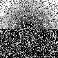
as well as the true underlying image that we would like to recover:

Each pixel in the image corresponds to a random variable whose unknown is the true pixel color. The goal is to use the neighborhood of each pixel to improve our estimate and resolve the original image. The synthetic_image_data application will also create the two input files needed to run the structured prediction application. The first is synthetic prior estimates for each pixel. Each row begins with the random variable id followed by the prior probability distribution for that random variable. Notice that the prior assigns half of the mass to the observed pixel value and the remaining mass to the other candidate pixel values.
> head synth_vdata.tsv
0 0.125 0.5 0.125 0.125 0.125
1 0.125 0.125 0.125 0.125 0.125
2 0.125 0.125 0.5 0.125 0.125
3 0.125 0.125 0.125 0.125 0.5
4 0.125 0.125 0.125 0.125 0.5
The second synth_edata.tsv file contains the graph structure with each line corresponding to an edge. Here we do not assign edge weights (and so the default weight of 1) will be used on all edges. Had we wanted to use weighted edges we would have added the weight value after each edge.
> head synth_edata.tsv
0 65536
0 1
1 65537
1 2
2 65538
2 3
We can now run the structured prediction application on the synthetic image.
> ./lbp_structured_prediction --prior synth_vdata.tsv --graph synth_edata.tsv \
                          --output posterior_vdata.tsv
Once the application terminates the final predictions will be stored in the sequence of files posterior_vdata.tsv_X_of_X in exactly the same format as the prior synth_vdata.tsv.
> ls -l posterior_vdata.tsv_*
posterior_vdata.tsv_1_of_2
posterior_vdata.tsv_2_of_2
in the format:
> head posterior_vdata.tsv_1_of_2
0 0.0237064 0.0947784 0.0245065 0.0323516 0.824657
1 0.00886895  0.0176509 0.0114683 0.0112453 0.950767
2 0.00402855  0.00489077  0.0161093 0.00426689  0.970705
3 0.00088747  0.00091284  0.00124409  0.000894688 0.996061
4 0.000696577 0.000695895 0.000706134 0.000695375 0.997206
5 0.000740404 0.000705437 0.000706437 0.000705451 0.997142
To visualize the predictions for the synthetic application we run:
> cat posterior_vdata.tsv_* | ./synthetic_image_data --pred pred_image.jpeg
Create a synthetic noisy image.
Reading in predictions
nrows: 200
ncols: 200
minp:  0
maxp:  4
If we then open pred_image.jpeg we get:

Not bad!
Dual Decomposition (DD), also called Lagrangian Relaxation, is a powerful technique with a rich history in Operations Research. DD solves a relaxation of difficult optimization problems by decomposing them into simpler subproblems, solving these simpler subproblems independently and then combining these solutions into an approximate global solution.
More details about DD for solving Maximum A Posteriori (MAP) inference problems in Markov Random Fields (MRFs) can be found in the following:
D. Sontag, A. Globerson, T. Jaakkola.
Introduction to Dual Decomposition for Inference.
Optimization for Machine Learning, editors S. Sra, S. Nowozin, and S. J. Wright: MIT Press, 2011.
Implemented by Andre' F. T. Martins and Dhruv Batra.
The input MRF graph is assumed to be in the standard UAI file format. For example a 3x3 grid MRF can be found here: grid3x3.uai.
The program can be run like this:
> ./dd --graph grid3x3.uai
Other arguments are:
 1.8.1.1
