Raster Symbolizer¶

Introduction¶

GeoServer supports the ability to display raster data in addition to vector data.

Raster data is not merely a picture, rather it can be thought of as a grid of georeferenced information, much like a graphic is a grid of visual information (with combination of reds, greens, and blues). Unlike graphics, which only contain visual data, each point/pixel in a raster grid can have lots of different attributes, with possibly none of them having an inherently visual component.

With the above in mind, one needs to choose how to visualize the data, and this, like in all other cases, is done by using an SLD. The analogy to vector data is evident in the naming of the tags used. Vectors, consisting of points, line, and polygons, are styled by using the <PointSymbolizer>, <LineSymbolizer>, and <PolygonSymbolizer> tags. It is therefore not very surprising that raster data is styled with the tag <RasterSymbolizer>.

Elements and Syntax¶

The following elements are available to be used as parameters inside <RasterSymbolizer>.

• <Opacity>
• <ColorMap>
• <ChannelSelection>
• <ContrastEnhancement>
• <ShadedRelief>
• <OverlapBehavior>
• <ImageOutline>

Notice that not all the above are actually implemented in the current version of the GeoServer.

Opacity¶

This element sets the transparency level for the entire dataset. As is standard, the values range from zero (0) to one (1), with zero being totally transparent, and one being not transparent at all. The syntax for <Opacity> is very simple:

<Opacity>0.5</Opacity>

where, in this case, the raster would be displayed at 50% opacity.

ColorMap¶

The <ColorMap> element sets rules for color gradients based on the quantity attribute. This quantity refers to the magnitude of the value of a data point. At its simplest, one could create two color map entries (the element called <ColorMapEntry>, one with a color for the “bottom” of the dataset, and another with a color for the “top” of the dataset. The colors in between will be automatically interpolated with the quantity values in between, making creating color gradients easy. One can also fine tune the color map by adding additional entries, which is handy if the dataset has more discrete values rather than a gradient. In that case, one could add an entry for each value to be set to a different color. In all cases, the color is denoted in standard hexadecimal RGB format (#RRGGBB). In addition to color and quantity, ColorMapEntry elements can also have opacity and label, the former which could be used instead of the global value mentioned previously, and the latter which could beused for legends.

For example a simple ColorMap can be:

<ColorMap>
        <ColorMapEntry color="#323232" quantity="-300" label="label1" opacity="1"/>
        <ColorMapEntry color="#BBBBBB" quantity="200" label="label2" opacity="1"/>
</ColorMap>

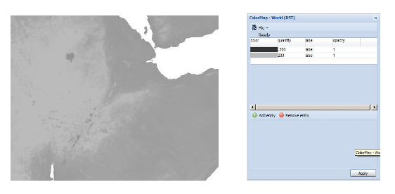
This example would create a color gradient from #323232 color to #BBBBBB color using quantity values -300 to 200:

<ColorMap>
        <ColorMapEntry color="#FFCC32" quantity="-300" label="label1" opacity="0"/>
        <ColorMapEntry color="#3645CC" quantity="0" label="label2" opacity="1"/>
        <ColorMapEntry color="#CC3636" quantity="100" label="label3" opacity="1"/>
        <ColorMapEntry color="#BBBBBB" quantity="200" label="label4" opacity="1"/>
</ColorMap>

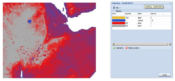
This example would create a color gradient from #FFCC32 color through #BBBBBB color running through #3645CC color and #CC3636 color. Here, though, #FFCC32 color would be transparent (simulating an alpha channel). Notice that default opacity, when not specified, is 1, which means opaque.

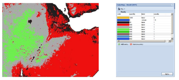
Two attributes can be created in ColorMap root node like ‘type’ and ‘extended’.

The ‘type’ attribute specifies the kind of ColorMap to use. There are three different types of ColorMaps that can be specified througth this attribute: ramp, intervals and values.

The ‘ramp’ is the default ColorMap type and the outcome is like the one presented at the beginning of this section (if into the ColorMap tag the attribute ‘type’ is not specified, the default value is ‘ramp’).

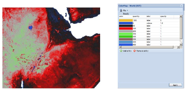
The ‘values’ means that only the specified entry quantities will be rendered, i.e. no color interpolation is applied between the entries.

The following example can clarify this aspect:

<ColorMap type="values">
        <ColorMapEntry color="#EEBE2F" quantity="-300" label="label" opacity="0"/>
        <ColorMapEntry color="#2851CC" quantity="0" label="values" opacity="1"/>
        <ColorMapEntry color="#211F1F" quantity="50" label="label" opacity="1"/>
        <ColorMapEntry color="#EE0F0F" quantity="100" label="label" opacity="1"/>
        <ColorMapEntry color="#AAAAAA" quantity="200" label="label" opacity="1"/>
        <ColorMapEntry color="#6FEE4F" quantity="250" label="label" opacity="1"/>
        <ColorMapEntry color="#3ECC1B" quantity="300" label="label" opacity="1"/>
        <ColorMapEntry color="#886363" quantity="350" label="label" opacity="1"/>
        <ColorMapEntry color="#5194CC" quantity="400" label="label" opacity="1"/>
        <ColorMapEntry color="#2C58DD" quantity="450" label="label" opacity="1"/>
        <ColorMapEntry color="#DDB02C" quantity="600" label="label" opacity="1"/>
</ColorMap>

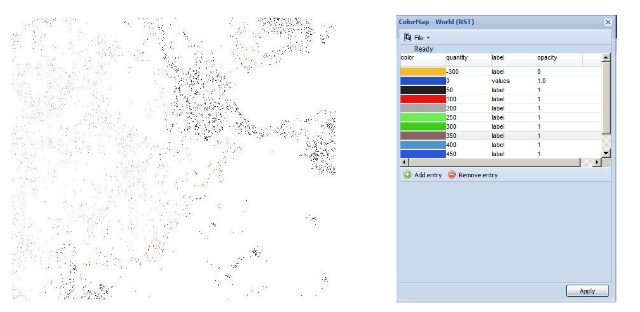
The ‘intervals’ value means that every interval defined by two entries will be colorized using the value of the first entrie, i.e. no color interpolation is applied between the intervals:

<ColorMap type="intervals" extended="true">
        <ColorMapEntry color="#EEBE2F" quantity="-300" label="label" opacity="0"/>
        ...
        <ColorMapEntry color="#DDB02C" quantity="600" label="label" opacity="1"/>
</ColorMap>

The ‘extended’ attribute allows ColorMap to compiute gradients using 256 or 65536 colors; extended=false means that the color scale is calculated on 8 bit, else 16 bit if the value is true.

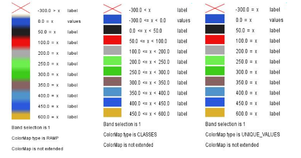
The difference between ramp, values and intervals values is also visible into raster legend. In order to get the raster legend from GeoServer the typically request is:

http://localhost:8080/geoserver/wms?REQUEST=GetLegendGraphic&VERSION=1.0.0&&STYLE=raster100&FORMAT=image/png&WIDTH=50&HEIGHT=20&LEGEND_OPTIONS=forceRule:true&LAYER=it.geosolutions:di08032_da

the results are:

ChannelSelection¶

This element specifies which color channel to access in the dataset. A dataset may contain standard three-channel colors (red, green, and blue channels) or one grayscale channel. Using <ChannelSelection> allows the mapping of a dataset channel to either a red, green, blue, or gray channel:

<ChannelSelection>
        <RedChannel>
        <SourceChannelName>1</SourceChannelName>
        </RedChannel>
        <GreenChannel>
        <SourceChannelName>2</SourceChannelName>
        </GreenChannel>
        <BlueChannel>
        <SourceChannelName>3</SourceChannelName>
        </BlueChannel>
</ChannelSelection>

The above would map source channels 1, 2,and 3 to the red, green, and blue Channels, respectively.

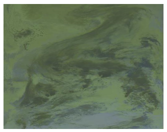
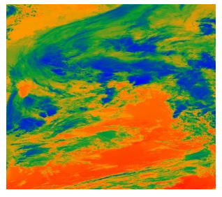
This is the result of gray ChannelSelection operation applied to an RGB image and re-colorized through a ColorMap:

<RasterSymbolizer>
        <Opacity>1.0</Opacity>
        <ChannelSelection>
                <GrayChannel>
                        <SourceChannelName>11</SourceChannelName>
                </GrayChannel>
        </ChannelSelection>
        <ColorMap extended="true">
                <ColorMapEntry color="#0000ff" quantity="3189.0"/>
                <ColorMapEntry color="#009933" quantity="6000.0"/>
                <ColorMapEntry color="#ff9900" quantity="9000.0" />
                <ColorMapEntry color="#ff0000" quantity="14265.0"/>
        </ColorMap>
</RasterSymbolizer>

ContrastEnhancement¶

The <ContrastEnhancement> element is used in color channels to adjust the relative brightness of the data in that channel. There are three types of enhancements possible.

• Normalize
• Histogram
• GammaValue

Normalize means to expand the contrast so that the minimum quantity is mapped to minimum brightness, and the maximum quantity is mapped to maximum brightness. Histogram is similar to Normalize, but the algorithm used attempts to produce an image with an equal number of pixels at all brightness levels. Finally, GammaValue is a scaling factor that adjusts the brightness of the data, with a value less than one (1) darkening the image, and a value greater than one (1) brightening it. (Normalize and Histogram do not have any parameters.) One can use <ContrastEnhancement> on a specific channel (say red only) as opposed to globally, if it is desired. In this way, different enhancements can be used on each channel:

<ContrastEnhancement>
        <Normalize/>
</ContrastEnhancement>

<ContrastEnhancement>
        <Histogram/>
</ContrastEnhancement>

These examples turn on Normalize and Histogram, respectively:

<ContrastEnhancement>
        <GammaValue>2</GammaValue>
</ContrastEnhancement>

The above increases the brightness of the data by a factor of two.

ShadedRelief¶

The <ShadedRelief> element can be used to create a 3-D effect, by selectively adjusting brightness. This is a nice effect to use on an elevation dataset. There are two types of shaded relief possible.

• BrightnessOnly
• ReliefFactor

BrightnessOnly, which takes no parameters, applies shading in WHAT WAY? ReliefFactor sets the amount of exaggeration of the shading (for example, to make hills appear higher). According to the OGC SLD specification, a value of around 55 gives “reasonable results” for Earth-based datasets:

<ShadedRelief>
        <BrightnessOnly />
        <ReliefFactor>55</ReliefFactor>
</ShadedRelief>

The above example turns on Relief shading in WHAT WAY?

OverlapBehavior¶

Sometimes raster data is comprised of multiple image sets. Take, for example, a satellite view of the Earth at night . As all of the Earth can’t be in nighttime at once, a composite of multiple images are taken. These images are georeferenced, and pieced together to make the finished product. That said, it is possible that two images from the same dataset could overlap slightly, and the OverlapBehavior element is designed to determine how this is handled. There are four types of OverlapBehavior:

• AVERAGE
• RANDOM
• LATEST_ON_TOP
• EARLIEST_ON_TOP

AVERAGE takes each overlapping point and displays their average value. RANDOM determines which image gets displayed according to chance (which can sometimes result in a crisper image). LATEST_ON_TOP and EARLIEST_ON_TOP sets the determining factor to be the internal timestamp on each image in the dataset. None of these elements have any parameters, and are all called in the same way:

<OverlapBehavior>
        <AVERAGE />
</OverlapBehavior>

The above sets the OverlapBehavior to AVERAGE.

ImageOutline¶

Given the situation mentioned previously of the image composite, it is possible to style each image so as to have an outline. One can even set a fill color and opacity of each image; a reason to do this would be to “gray-out” an image. To use ImageOutline, you would define a <LineSymbolizer> or <PolygonSymbolizer> inside of the element:

<ImageOutline>
        <LineSymbolizer>
        <Stroke>
                        <CssParameter name="stroke">#0000ff</CssParameter>
        </Stroke>
        </LineSymbolizer>
</ImageOutline>

The above would create a border line (colored blue with a one pixel default thickness) around each image in the dataset.