12 Linguistic Data Management (DRAFT)
12.1 Introduction
Language resources of all kinds are proliferating on the Web. These include data such as lexicons and annotated text, and software tools for creating and manipulating the data. As we have seen in previous chapters, language resources are essential in most areas of NLP. This has been made possible by three significant technological developments over the past decade. First, inexpensive mass storage technology permits large resources to be stored in digital form, while the Extensible Markup Language (XML) and Unicode provide flexible ways to represent structured data and give it good prospects for long-term survival. Second, digital publication has been a practical and efficient means of sharing language resources. Finally, search engines, mailing lists, and online resource catalogs make it possible for people to discover the existence of the resources they may be seeking.
Together with these technological advances have been three other developments that have shifted the NLP community in the direction of data-intensive approaches. First, the "shared task method," an initiative of government sponsors, supports major sections within the community to identify a common goal for the coming year, and provides "gold standard" data on which competing systems can be evaluated. Second, data publishers such as the Linguistic Data Consortium have negotiated with hundreds of data providers (including newswire services in many countries), and created hundreds of annotated corpora stored in well-defined and consistent formats. Finally, organizations that purchase NLP systems, or that publish NLP papers, now expect the quality of the work to be demonstrated using standard datasets.
Although language resources are central to NLP, we still face many obstacles in using them. First, the resource we are looking for may not exist, and so we have to think about creating a new language resource, and doing a sufficiently careful job that it serves our future needs, thanks to its coverage, balance, and documentation of the sources. Second, a resource may exist but its creator didn't document its existence anywhere, leaving us to recreate the resource; however, to save further wasted effort we should learn about publishing metadata the documents the existence of a resource, and even how to publish the resource itself, in a form that is easy for others to re-use. Third, the resource may exist and may be obtained, but is in an incompatible format, and so we need to set about converting the data into a different format. Finally, the resource may be in the right format, but the available software is unable to perform the required analysis task, and so we need to develop our own program for analyzing the data. This chapter covers each of these issues — creating, publishing, converting, and analyzing — using many examples drawn from practical experience managing linguistic data. However, before embarking on this sequence of issues, we start by examining the organization of linguistic data.
12.2 Linguistic Databases
Linguistic databases span a multidimensional space of cases, which we can divide up in several ways: the scope and design of the data collection; the goals of the creators; the nature of the material included; the goals and methods of the users (which are often not anticipated by the creators). Three examples follow.
In one type of linguistic database, the design unfolds interactively in the course of the creator's explorations. This is the pattern typical of traditional "field linguistics," in which material from elicitation sessions is analyzed repeatedly as it is gathered, with tomorrow's elicitation often based on questions that arise in analyzing today's. The resulting field notes are then used during subsequent years of research, and may serve as an archival resource indefinitely — the field notes of linguists and anthropologists working in the early years of the 20th century remain an important source of information today. Computerization is an obvious boon to work of this type, as exemplified by the popular program Shoebox — now about two decades old and re-released as Toolbox — which replaces the field linguist's traditional shoebox full of file cards.
Another pattern is represented by experimental approaches in which a body of carefully-designed material is collected from a range of subjects, then analyzed to evaluate a hypothesis or develop a technology. Today, such databases are collected and analyzed in digital form. Among scientists (such as phoneticians or psychologists), they are rarely published and therefore rarely preserved. Among engineers, it has become common for such databases to be shared and re-used at least within a laboratory or company, and often to be published more widely. Linguistic databases of this type are the basis of the "common task" method of research management, which over the past 15 years has become the norm in government-funded research programs in speech- and language-related technology.
Finally, there are efforts to gather a "reference corpus" for a particular language. Large and well-documented examples include the American National Corpus (ANC) and the British National Corpus (BNC). The goal in such cases is to produce a set of linguistic materials that cover the many forms, styles and uses of a language as widely as possible. The core application is typically lexicographic, that is, the construction of dictionaries based on a careful study of patterns of use. These corpora were constructed by large consortia spanning government, industry, and academia. Their planning and execution took more than five years, and indirectly involved hundreds of person-years of effort. There is also a long and distinguished history of other humanistic reference corpora, such the Thesaurus Linguae Graecae.
There are no hard boundaries among these categories. Accumulations of smaller bodies of data may come in time to constitute a sort of reference corpus, while selections from large databases may form the basis for a particular experiment. Further instructive examples follow.
A linguist's field notes may include extensive examples of many genres (proverbs, conversations, narratives, rituals, and so forth), and may come to constitute a reference corpus of modest but useful size. There are many extinct languages for which such material is all the data we will ever have, and many more endangered languages for which such documentation is urgently needed. Sociolinguists typically base their work on analysis of a set of recorded interviews, which may over time grow to create another sort of reference corpus. In some labs, the residue of decades of work may comprise literally thousands of hours of recordings, many of which have been transcribed and annotated to one extent or another. The CHILDES corpus, comprising transcriptions of parent-child interactions in many languages, contributed by many individual researchers, has come to constitute a widely-used reference corpus for language acquisition research. Speech technologists aim to produce training and testing material of broad applicability, and wind up creating another sort of reference corpus. To date, linguistic technology R&D has been the primary source of published linguistic databases of all sorts (see e.g. http://www.ldc.upenn.edu/).
As large, varied linguistic databases are published, phoneticians or psychologists are increasingly likely to base experimental investigations on balanced, focused subsets extracted from databases produced for entirely different reasons. Their motivations include the desire to save time and effort, the desire to work on material available to others for replication, and sometimes a desire to study more naturalistic forms of linguistic behavior. The process of choosing a subset for such a study, and making the measurements involved, is usually in itself a non-trivial addition to the database. This recycling of linguistic databases for new purposes is a normal and expected consequence of publication. For instance, the Switchboard database, originally collected for speaker identification research, has since been used as the basis for published studies in speech recognition, word pronunciation, disfluency, syntax, intonation and discourse structure.
At present, only a tiny fraction of the linguistic databases that are collected are published in any meaningful sense. This is mostly because publication of such material was both time-consuming and expensive, and because use of such material by other researchers was also both expensive and technically difficult. However, general improvements in hardware, software and networking have changed this, and linguistic databases can now be created, published, stored and used without inordinate effort or large expense.
In practice, the implications of these cost-performance changes are only beginning to be felt. The main problem is that adequate tools for creation, publication and use of linguistic data are not widely available. In most cases, each project must create its own set of tools, which hinders publication by researchers who lack the expertise, time or resources to make their data accessible to others. Furthermore, we do not have adequate, generally accepted standards for expressing the structure and content of linguistic databases. Without such standards, general-purpose tools are impossible — though at the same time, without available tools, adequate standards are unlikely to be developed, used and accepted. Just as importantly, there must be a critical mass of users and published material to motivate maintenance of data and access tools over time.
Relative to these needs, the present chapter has modest goals, namely to equip readers to take linguistic databases into their own hands by writing programs to help create, publish, transform and analyze the data. In the rest of this section we take a close look at the fundamental data types, an exemplary speech corpus, and the lifecycle of linguistic data.
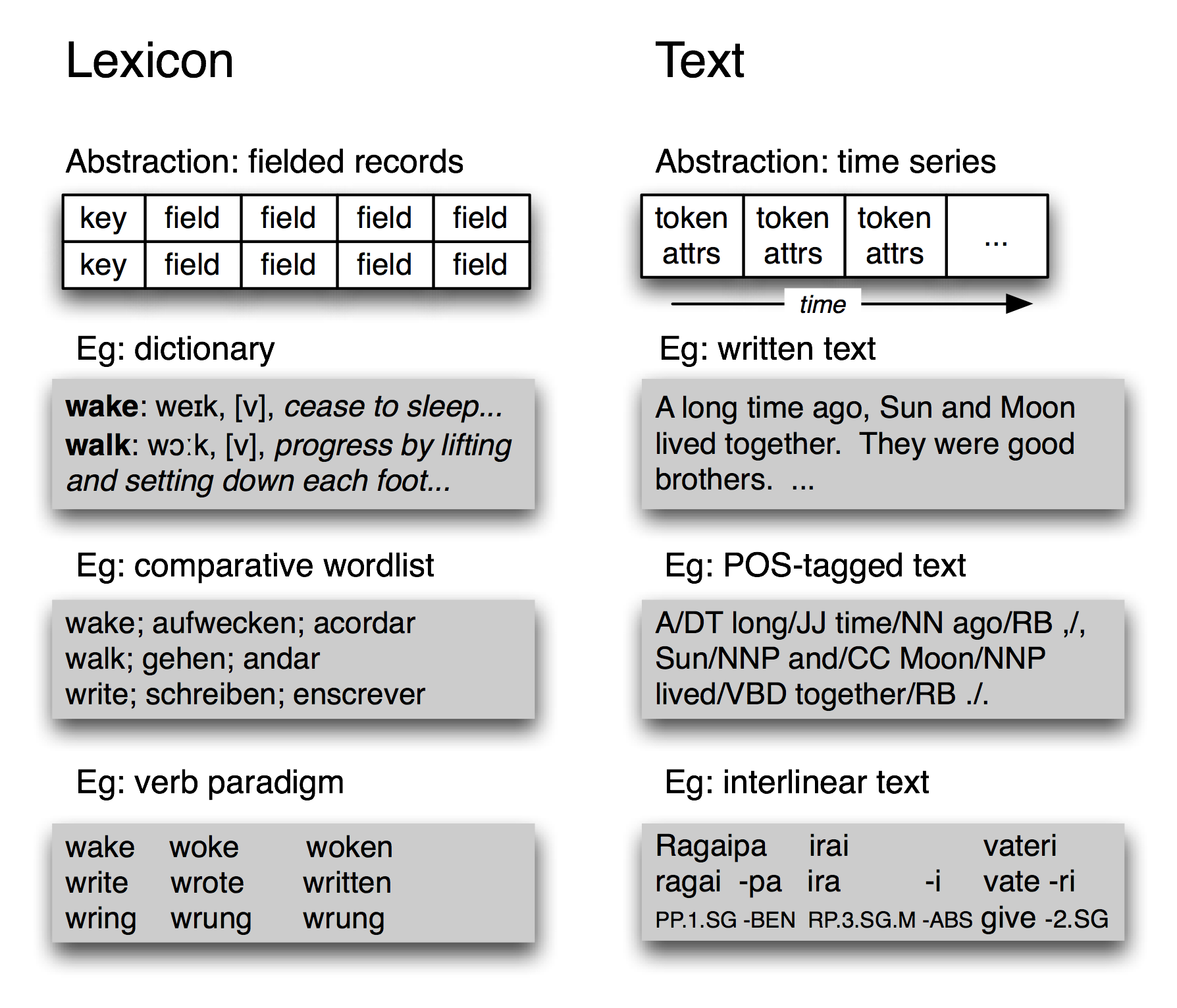
Figure 12.1: Basic Linguistic Datatypes: Lexicons and Texts
12.2.1 Fundamental Data Types
Linguistic data management deals with a variety of data types, the most important being lexicons and texts. A lexicon is a database of words, minimally containing part of speech information and glosses. For many lexical resources, it is sufficient to use a record structure, i.e. a key plus one or more fields, as shown in Figure 12.1. A lexical resource could be a conventional dictionary or comparative wordlist, as illustrated. Several related linguistic data types also fit this model. For example in a phrasal lexicon, the key field is a phrase rather than a single word. A thesaurus can be derived from a lexicon by adding topic fields to the entries and constructing an index over those fields. We can also construct special tabulations (known as paradigms) to illustrate contrasts and systematic variation, as shown in Figure 12.1 for three verbs.
At the most abstract level, a text is a representation of a real or fictional speech event, and the time-course of that event carries over into the text itself. A text could be a small unit, such as a word or sentence, or a complete narrative or dialogue. It may come with annotations such as part-of-speech tags, morphological analysis, discourse structure, and so forth. As we saw in the IOB tagging technique (Chapter 6), it is possible to represent higher-level constituents using tags on individual words. Thus the abstraction of text shown in Figure 12.1 is sufficient.
12.2.2 Corpus Structure: a Case Study of TIMIT
The TIMIT corpus of read speech was the first annotated speech database to be widely distributed, and it has an especially clear organization. TIMIT was developed by a consortium including Texas Instruments and MIT (hence the name), and was designed to provide data for the acquisition of acoustic-phonetic knowledge and to support the development and evaluation of automatic speech recognition systems.
Like the Brown Corpus, which displays a balanced selection of text genres and sources, TIMIT includes a balanced selection of dialects, speakers, and materials. For each of eight dialect regions, 50 male and female speakers having a range of ages and educational backgrounds each read ten carefully chosen sentences. Two sentences, read by all speakers, were designed to bring out dialect variation:
| (1) |
|
The remaining sentences were chosen to be phonetically rich, involving all phones (sounds) and a comprehensive range of diphones (phone bigrams). Additionally, the design strikes a balance between multiple speakers saying the same sentence in order to permit comparison across speakers, and having a large range of sentences covered by the corpus to get maximal coverage of diphones. Thus, five sentences read by each speaker, are also read by six other speakers (comparability). The remaining three sentences read by each speaker were unique to that speaker (coverage).
NLTK includes a sample from the TIMIT corpus. You can access its documentation in the usual way, using help(corpus.timit). Print corpus.timit.items to see a list of the 160 recorded utterances in the corpus sample. Each item name has complex internal structure, as shown in Figure 12.2.
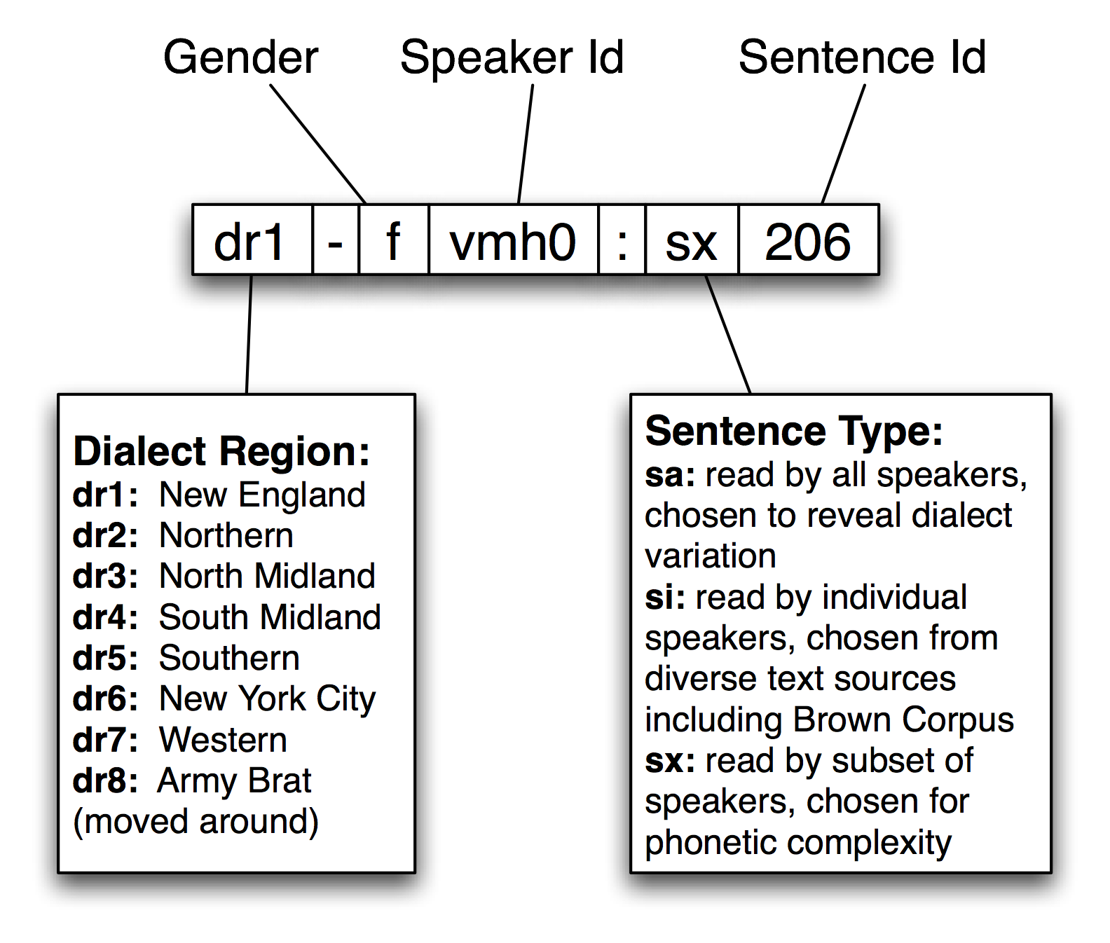
Figure 12.2: Structure of a TIMIT Identifier in the NLTK Corpus Package
Each item has a phonetic transcription, which can be accessed using the phones() method. We can access the corresponding word tokens in the customary way. Both access methods permit an optional argument offset=True which includes the start and end offsets of the corresponding span in the audio file.
|
Note
Remember that our program samples assume you begin your interactive session or your program with: import nltk, re, pprint (Note that some of the examples in this chapter have not yet been updated to work with NLTK-Lite version 0.9).
In addition to this text data, TIMIT includes a lexicon that provides the canonical pronunciation of every word:
|
This gives us a sense of what a speech processing system would have to do in producing or recognizing speech in this particular dialect (New England). Finally, TIMIT includes demographic data about the speakers, permitting fine-grained study of vocal, social, and gender characteristics.
|
TIMIT illustrates several key features of corpus design. First, the corpus contains two layers of annotation, at the phonetic and orthographic levels. In general, a text or speech corpus may be annotated at many different linguistic levels, including morphological, syntactic, and discourse levels. Moreover, even at a given level there may be different labeling schemes or even disagreement amongst annotators, such that we want to represent multiple versions. A second property of TIMIT is its balance across multiple dimensions of variation, for coverage of dialect regions and diphones. The inclusion of speaker demographics brings in many more independent variables, that may help to account for variation in the data, and which facilitate later uses of the corpus for purposes that were not envisaged when the corpus was created, e.g. sociolinguistics. A third property is that there is a sharp division between the original linguistic event captured as an audio recording, and the annotations of that event. The same holds true of text corpora, in the sense that the original text usually has an external source, and is considered to be an immutable artifact. Any transformations of that artifact which involve human judgment — even something as simple as tokenization — are subject to later revision, thus it is important to retain the source material in a form that is as close to the original as possible.
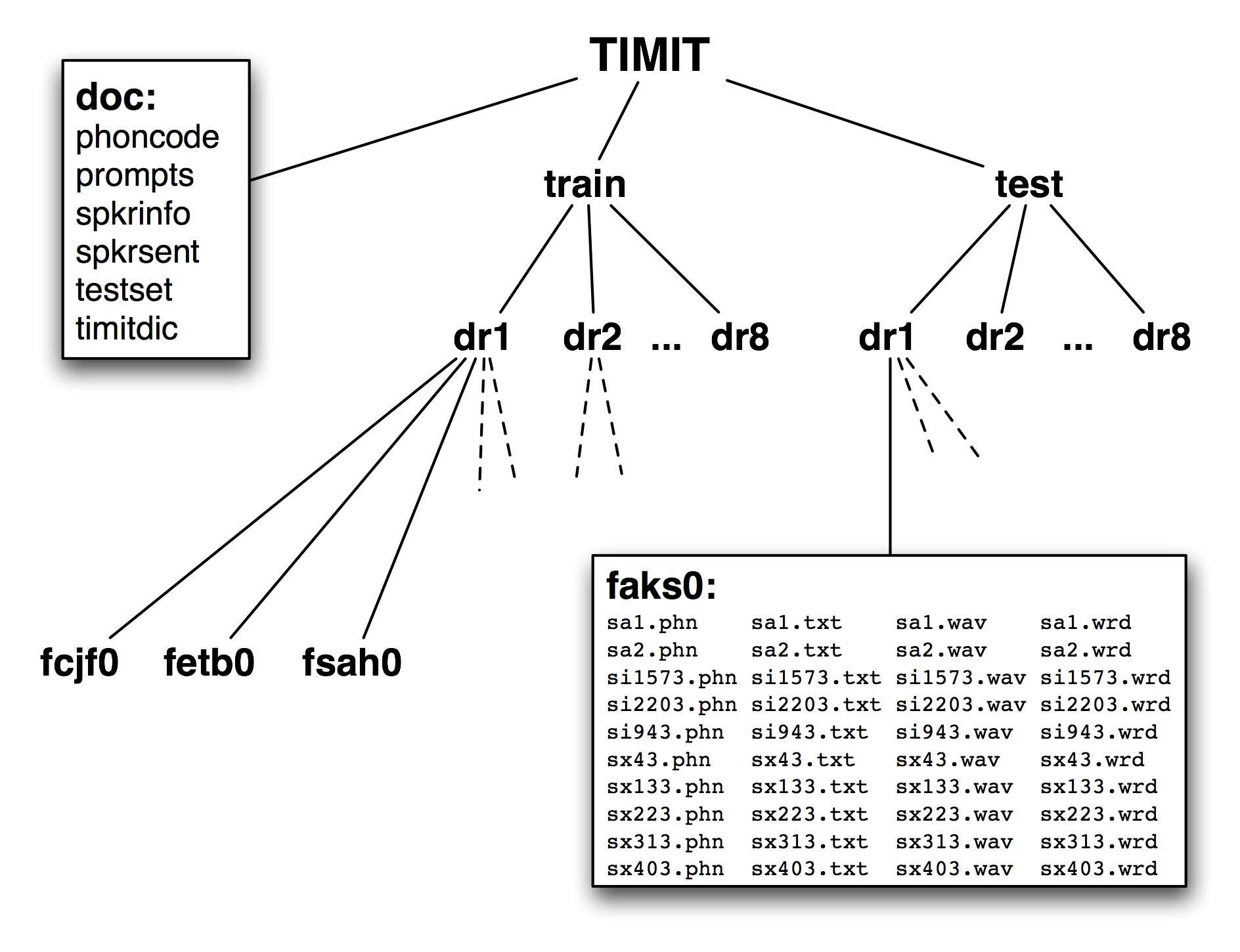
Figure 12.3: Structure of the Published TIMIT Corpus
A fourth feature of TIMIT is the hierarchical structure of the corpus. With 4 files per sentence, and 10 sentences for each of 500 speakers, there are 20,000 files. These are organized into a tree structure, shown schematically in Figure 12.3. At the top level there is a split between training and testing sets, which gives away its intended use for developing and evaluating statistical models.
Finally, notice that even though TIMIT is a speech corpus, its transcriptions and associated data are just text, and can be processed using programs just like any other text corpus. Therefore, many of the computational methods described in this book are applicable. Moreover, notice that all of the data types included in the TIMIT corpus fall into our two basic categories of lexicon and text (cf. section 12.2.1). Even the speaker demographics data is just another instance of the lexicon data type.
This last observation is less surprising when we consider that text and record structures are the primary domains for the two subfields of computer science that focus on data management, namely text retrieval and databases. A notable feature of linguistic data management is that usually brings both data types together, and that it can draw on results and techniques from both fields.
12.2.3 The Lifecycle of Linguistic Data: Evolution vs Curation
Once a corpus has been created and disseminated, it typically gains a life of its own, as others adapt it to their needs. This may involve reformatting a text file (e.g. converting to XML), renaming files, retokenizing the text, selecting a subset of the data to enrich, and so forth. Multiple research groups may do this work independently, as exemplified in Figure 12.4. At a later date, when someone wants to combine sources of information from different version, the task may be extremely onerous.
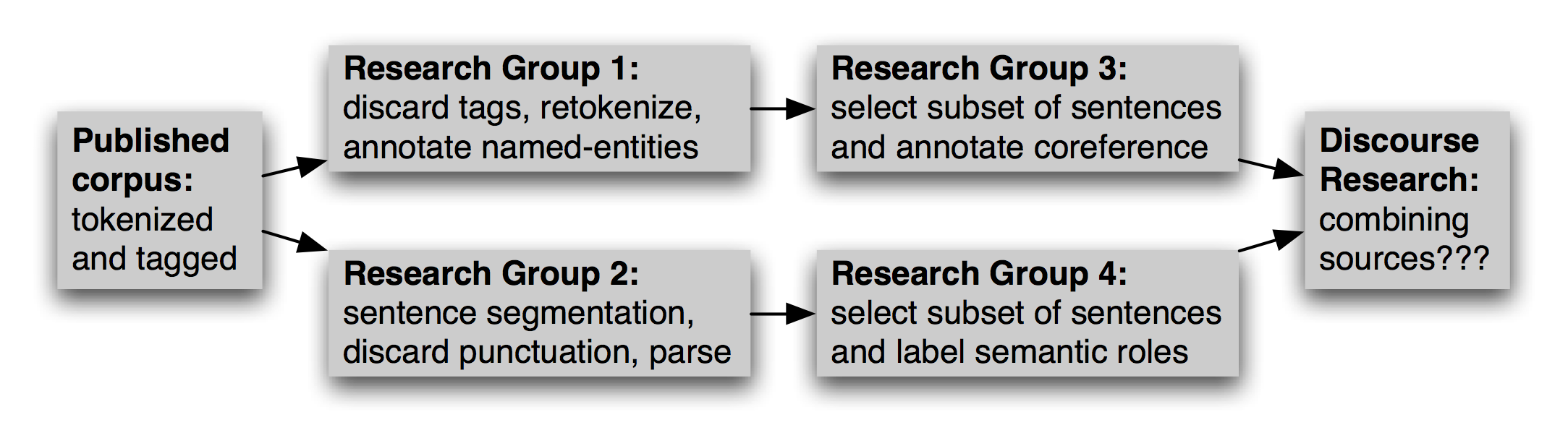
Figure 12.4: Evolution of a Corpus
The task of using derived corpora is made even more difficult by the lack of any record about how the derived version was created, and which version is the most up-to-date.
An alternative to this chaotic situation is for all corpora to be centrally curated, and for committees of experts to revise and extend a reference corpus at periodic intervals, considering proposals for new content from third-parties, much like a dictionary is edited. However, this is impractical.
A better solution is to have a canonical, immutable primary source, which supports incoming references to any sub-part, and then for all annotations (including segmentations) to reference this source. This way, two independent tokenizations of the same text can be represented without touch the source text, as can any further labeling and grouping of those annotations. This method is known as standoff annotation.
[More discussion and examples]
12.3 Creating Data
Scenarios: fieldwork, web, manual entry using local tool, machine learning with manual post-editing
Conventional office software is widely used in computer-based language documentation work, given its familiarity and ready availability. This includes word processors and spreadsheets.
12.3.1 Spiders
- what they do: basic idea is simple
- python code to find all the anchors, extract the href, and make an absolute URL for fetching
- many issues: starting points, staying within a single site, only getting HTML
- various stand-alone tools for spidering, and mirroring
12.3.2 Creating Language Resources Using Word Processors
Word processing software is often used in creating dictionaries and interlinear texts. As the data grows in size and complexity, a larger proportion of time is spent maintaining consistency. Consider a dictionary in which each entry has a part-of-speech field, drawn from a set of 20 possibilities, displayed after the pronunciation field, and rendered in 11-point bold. No conventional word processor has search or macro functions capable of verifying that all part-of-speech fields have been correctly entered and displayed. This task requires exhaustive manual checking. If the word processor permits the document to be saved in a non-proprietary format, such as text, HTML, or XML, we can sometimes write programs to do this checking automatically.
Consider the following fragment of a lexical entry: "sleep [sli:p] vi condition of body and mind...". We can enter this in MSWord, then "Save as Web Page", then inspect the resulting HTML file:
<p class=MsoNormal>sleep
  <span style='mso-spacerun:yes'> </span>
  [<span class=SpellE>sli:p</span>]
  <span style='mso-spacerun:yes'> </span>
  <b><span style='font-size:11.0pt'>vi</span></b>
  <span style='mso-spacerun:yes'> </span>
  <i>a condition of body and mind ...<o:p></o:p></i>
</p>
Observe that the entry is represented as an HTML paragraph, using the <p> element, and that the part of speech appears inside a <span style='font-size:11.0pt'> element. The following program defines the set of legal parts-of-speech, legal_pos. Then it extracts all 11-point content from the dict.htm file and stores it in the set used_pos. Observe that the search pattern contains a parenthesized sub-expression; only the material that matches this sub-expression is returned by re.findall. Finally, the program constructs the set of illegal parts-of-speech as used_pos - legal_pos:
|
This simple program represents the tip of the iceberg. We can develop sophisticated tools to check the consistency of word processor files, and report errors so that the maintainer of the dictionary can correct the original file using the original word processor.
We can write other programs to convert the data into a different format. For example, Listing 12.1 strips out the HTML markup using ntlk.clean_html(), extracts the words and their pronunciations, and generates output in "comma-separated value" (CSV) format:
| ||
| ||
Listing 12.1 (html2csv.py): Converting HTML Created by Microsoft Word into Comma-Separated Values |
12.3.3 Creating Language Resources Using Spreadsheets and Databases
Spreadsheets. These are often used for wordlists or paradigms. A comparative wordlist may be stored in a spreadsheet, with a row for each cognate set, and a column for each language. Examples are available from www.rosettaproject.org. Programs such as Excel can export spreadsheets in the CSV format, and we can write programs to manipulate them, with the help of Python's csv module. For example, we may want to print out cognates having an edit-distance of at least three from each other (i.e. 3 insertions, deletions, or substitutions).
Databases. Sometimes lexicons are stored in a full-fledged relational database. When properly normalized, these databases can implement many well-formedness constraints. For example, we can require that all parts-of-speech come from a specified vocabulary by declaring that the part-of-speech field is an enumerated type. However, the relational model is often too restrictive for linguistic data, which typically has many optional and repeatable fields (e.g. dictionary sense definitions and example sentences). Query languages such as SQL cannot express many linguistically-motivated queries, e.g. find all words that appear in example sentences for which no dictionary entry is provided. Now supposing that the database supports exporting data to CSV format, and that we can save the data to a file dict.csv:
"sleep","sli:p","v.i","a condition of body and mind ..."
"walk","wo:k","v.intr","progress by lifting and setting down each foot ..."
"wake","weik","intrans","cease to sleep"
Now we can express this query as shown in Figure 12.2.
| ||
| ||
Listing 12.2 (undefined_words.py): Finding definition words not themselves defined |
12.3.4 Creating Language Resources Using Toolbox
Over the last two decades, several dozen tools have been developed that provide specialized support for linguistic data management. Perhaps the single most popular tool used by linguists for managing data is Toolbox, previously known as Shoebox (freely downloadable from http://www.sil.org/computing/toolbox/). In this section we discuss a variety of techniques for manipulating Toolbox data in ways that are not supported by the Toolbox software. (The methods we discuss could be applied to other record-structured data, regardless of the actual file format.)
A Toolbox file consists of a collection of entries (or records), where each record is made up of one or more fields. Here is an example of an entry taken from a Toolbox dictionary of Rotokas. (Rotokas is an East Papuan language spoken on the island of Bougainville; this data was provided by Stuart Robinson, and is a sample from a larger lexicon):
\lx kaa
\ps N
\pt MASC
\cl isi
\ge cooking banana
\tkp banana bilong kukim
\pt itoo
\sf FLORA
\dt 12/Aug/2005
\ex Taeavi iria kaa isi kovopaueva kaparapasia.
\xp Taeavi i bin planim gaden banana bilong kukim tasol long paia.
\xe Taeavi planted banana in order to cook it.
This lexical entry contains the following fields: lx lexeme; ps part-of-speech; pt part-of-speech; cl classifier; ge English gloss; tkp Tok Pisin gloss; sf Semantic field; dt Date last edited; ex Example sentence; xp Pidgin translation of example; xe English translation of example. These field names are preceded by a backslash, and must always appear at the start of a line. The characters of the field names must be alphabetic. The field name is separated from the field's contents by whitespace. The contents can be arbitrary text, and can continue over several lines (but cannot contain a line-initial backslash).
We can use the toolbox.xml() method to access a Toolbox file and load it into an elementtree object.
|
There are two ways to access the contents of the lexicon object, by indexes and by paths. Indexes use the familiar syntax, thus lexicon[3] returns entry number 3 (which is actually the fourth entry counting from zero). And lexicon[3][0] returns its first field:
|
The second way to access the contents of the lexicon object uses paths. The lexicon is a series of record objects, each containing a series of field objects, such as lx and ps. We can conveniently address all of the lexemes using the path record/lx. Here we use the findall() function to search for any matches to the path record/lx, and we access the text content of the element, normalizing it to lowercase.
|
It is often convenient to add new fields that are derived automatically from existing ones. Such fields often facilitate search and analysis. For example, in Listing 12.3 we define a function cv() which maps a string of consonants and vowels to the corresponding CV sequence, e.g. kakapua would map to CVCVCVV. This mapping has four steps. First, the string is converted to lowercase, then we replace any non-alphabetic characters [^a-z] with an underscore. Next, we replace all vowels with V. Finally, anything that is not a V or an underscore must be a consonant, so we replace it with a C. Now, we can scan the lexicon and add a new cv field after every lx field. Listing 12.3 shows what this does to a particular entry; note the last line of output, which shows the new CV field.
| ||
| ||
Listing 12.3 (add_cv_field.py): Adding a new cv field to a lexical entry |
Finally, we take a look at simple methods to generate summary reports, giving us an overall picture of the quality and organisation of the data.
First, suppose that we wanted to compute the average number of fields for each entry. This is just the total length of the entries (the number of fields they contain), divided by the number of entries in the lexicon:
|
| ||
| ||
Listing 12.4 (toolbox_validation.py): Validating Toolbox Entries Using a Context Free Grammar |
We could try to write down a grammar for lexical entries, and look for entries which do not conform to the grammar. In general, toolbox entries have nested structure. Thus they correspond to a tree over the fields. We can check for well-formedness by parsing the field names. In Listing 12.5 we set up a putative grammar for the entries, then parse each entry. Those that are accepted by the grammar prefixed with a '+', and those that are rejected are prefixed with a '-'.
| ||
| ||
Listing 12.5 (chunk_toolbox.py): Chunking a Toolbox Lexicon |
12.3.5 Interlinear Text
The NLTK corpus collection includes many interlinear text samples (though no suitable corpus reader as yet).
General Ontology for Linguistic Description (GOLD) http://www.linguistics-ontology.org/
12.3.6 Creating Metadata for Language Resources
OLAC metadata extends the Dublin Core metadata set with descriptors that are important for language resources.
The container for an OLAC metadata record is the element <olac>. Here is a valid OLAC metadata record from the Pacific And Regional Archive for Digital Sources in Endangered Cultures (PARADISEC):
<olac:olac xsi:schemaLocation="http://purl.org/dc/elements/1.1/ http://www.language-archives.org/OLAC/1.0/dc.xsd
  http://purl.org/dc/terms/ http://www.language-archives.org/OLAC/1.0/dcterms.xsd
  http://www.language-archives.org/OLAC/1.0/ http://www.language-archives.org/OLAC/1.0/olac.xsd">
  <dc:title>Tiraq Field Tape 019</dc:title>
  <dc:identifier>AB1-019</dc:identifier>
  <dcterms:hasPart>AB1-019-A.mp3</dcterms:hasPart>
  <dcterms:hasPart>AB1-019-A.wav</dcterms:hasPart>
  <dcterms:hasPart>AB1-019-B.mp3</dcterms:hasPart>
  <dcterms:hasPart>AB1-019-B.wav</dcterms:hasPart>
  <dc:contributor xsi:type="olac:role" olac:code="recorder">Brotchie, Amanda</dc:contributor>
  <dc:subject xsi:type="olac:language" olac:code="x-sil-MME"/>
  <dc:language xsi:type="olac:language" olac:code="x-sil-BCY"/>
  <dc:language xsi:type="olac:language" olac:code="x-sil-MME"/>
  <dc:format>Digitised: yes;</dc:format>
  <dc:type>primary_text</dc:type>
  <dcterms:accessRights>standard, as per PDSC Access form</dcterms:accessRights>
  <dc:description>SIDE A<p>1. Elicitation Session - Discussion and
    translation of Lise's and Marie-Claire's Songs and Stories from
    Tape 18 (Tamedal)<p><p>SIDE B<p>1. Elicitation Session: Discussion
    of and translation of Lise's and Marie-Clare's songs and stories
    from Tape 018 (Tamedal)<p>2. Kastom Story 1 - Bislama
    (Alec). Language as given: Tiraq</dc:description>
</olac:olac>
NLTK Version 0.9 includes support for reading an OLAC record, for example:
|
12.3.7 Linguistic Annotation
Annotation graph model
multiple overlapping trees over shared data
Large annotation tasks require multiple annotators. How consistently can a group of annotators perform? It is insufficient to report that there is 80% agreement, as we have no way to tell if this is good or bad. I.e. for an easy task such as tagging, this would be a bad score, while for a difficult task such as semantic role labeling, this would be an exceptionally good score.
The Kappa coefficient K measures agreement between two people making category judgments, correcting for expected chance agreement. For example, suppose an item is to be annotated, and four coding options are equally likely. Then people coding randomly would be expected to agree 25% of the time. Thus, an agreement of 25% will be assigned K = 0, and better levels of agreement will be scaled accordingly. For an agreement of 50%, we would get K = 0.333, as 50 is a third of the way from 25 to 100.
12.3.8 Exercises
- ☼ Write a program to filter out just the date field (dt) without having to list the fields we wanted to retain.
- ☼ Print an index of a lexicon. For each lexical entry, construct a tuple of the form (gloss, lexeme), then sort and print them all.
- ☼ What is the frequency of each consonant and vowel contained in lexeme fields?
- ◑ In Listing 12.3 the new field appeared at the bottom of the entry. Modify this program so that it inserts the new subelement right after the lx field. (Hint: create the new cv field using Element('cv'), assign a text value to it, then use the insert() method of the parent element.)
- ◑ Write a function that deletes a specified field from a lexical entry. (We could use this to sanitize our lexical data before giving it to others, e.g. by removing fields containing irrelevant or uncertain content.)
- ◑ Write a program that scans an HTML dictionary file to find entries having an illegal part-of-speech field, and reports the headword for each entry.
- ◑ Write a program to find any parts of speech (ps field) that occurred less than ten times. Perhaps these are typing mistakes?
- ◑ We saw a method for discovering cases of whole-word reduplication. Write a function to find words that may contain partial reduplication. Use the re.search() method, and the following regular expression: (..+)\1
- ◑ We saw a method for adding a cv field. There is an interesting issue with keeping this up-to-date when someone modifies the content of the lx field on which it is based. Write a version of this program to add a cv field, replacing any existing cv field.
- ◑ Write a function to add a new field syl which gives a count of the number of syllables in the word.
- ◑ Write a function which displays the complete entry for a lexeme. When the lexeme is incorrectly spelled it should display the entry for the most similarly spelled lexeme.
- ◑ Write a function that takes a lexicon and finds which pairs of consecutive fields are most frequent (e.g. ps is often followed by pt). (This might help us to discover some of the structure of a lexical entry.)
- ★ Obtain a comparative wordlist in CSV format, and write a program that prints those cognates having an edit-distance of at least three from each other.
- ★ Build an index of those lexemes which appear in example sentences. Suppose the lexeme for a given entry is w. Then add a single cross-reference field xrf to this entry, referencing the headwords of other entries having example sentences containing w. Do this for all entries and save the result as a toolbox-format file.
12.4 Converting Data Formats
- write our own parser and formatted print
- use existing libraries, e.g. csv
12.4.1 Formatting Entries
We can also print a formatted version of a lexicon. It allows us to request specific fields without needing to be concerned with their relative ordering in the original file.
|
We can use the same idea to generate HTML tables instead of plain text. This would be useful for publishing a Toolbox lexicon on the web. It produces HTML elements <table>, <tr> (table row), and <td> (table data).
|
XML output
|
12.4.2 Exercises
- ◑ Create a spreadsheet using office software, containing one lexical entry per row, consisting of a headword, a part of speech, and a gloss. Save the spreadsheet in CSV format. Write Python code to read the CSV file and print it in Toolbox format, using lx for the headword, ps for the part of speech, and gl for the gloss.
12.5 Analyzing Language Data
I.e. linguistic exploration
Export to statistics package via CSV
In this section we consider a variety of analysis tasks.
Reduplication: First, we will develop a program to find reduplicated words. In order to do this we need to store all verbs, along with their English glosses. We need to keep the glosses so that they can be displayed alongside the wordforms. The following code defines a Python dictionary lexgloss which maps verbs to their English glosses:
|
Next, for each verb lex, we will check if the lexicon contains the reduplicated form lex+lex. If it does, we report both forms along with their glosses.
|
Complex Search Criteria: Phonological description typically identifies the segments, alternations, syllable canon and so forth. It is relatively straightforward to count up the occurrences of all the different types of CV syllables that occur in lexemes.
In the following example, we first import the regular expression and probability modules. Then we iterate over the lexemes to find all sequences of a non-vowel [^aeiou] followed by a vowel [aeiou].
|
Now, rather than just printing the syllables and their frequency counts, we can tabulate them to generate a useful display.
|
Consider the t and s columns, and observe that ti is not attested, while si is frequent. This suggests that a phonological process of palatalization is operating in the language. We would then want to consider the other syllables involving s (e.g. the single entry having su, namely kasuari 'cassowary' is a loanword).
Prosodically-motivated search: A phonological description may include an examination of the segmental and prosodic constraints on well-formed morphemes and lexemes. For example, we may want to find trisyllabic verbs ending in a long vowel. Our program can make use of the fact that syllable onsets are obligatory and simple (only consist of a single consonant). First, we will encapsulate the syllabic counting part in a separate function. It gets the CV template of the word cv(word) and counts the number of consonants it contains:
|
We also encapsulate the vowel test in a function, as this improves the readability of the final program. This function returns the value True just in case char is a vowel.
|
Over time we may create a useful collection of such functions. We can save them in a file utilities.py, and then at the start of each program we can simply import all the functions in one go using from utilities import *. We take the entry to be a verb if the first letter of its part of speech is a V. Here, then, is the program to display trisyllabic verbs ending in a long vowel:
|
Finding Minimal Sets: In order to establish a contrast segments (or lexical properties, for that matter), we would like to find pairs of words which are identical except for a single property. For example, the words pairs mace vs maze and face vs faze — and many others like them — demonstrate the existence of a phonemic distinction between s and z in English. NLTK provides flexible support for constructing minimal sets, using the MinimalSet() class. This class needs three pieces of information for each item to be added: context: the material that must be fixed across all members of a minimal set; target: the material that changes across members of a minimal set; display: the material that should be displayed for each item.
| Examples of Minimal Set Parameters | |||
|---|---|---|---|
| Minimal Set | Context | Target | Display |
| bib, bid, big | first two letters | third letter | word |
| deal (N), deal (V) | whole word | pos | word (pos) |
We begin by creating a list of parameter values, generated from the full lexical entries. In our first example, we will print minimal sets involving lexemes of length 4, with a target position of 1 (second segment). The context is taken to be the entire word, except for the target segment. Thus, if lex is kasi, then context is lex[:1]+'_'+lex[2:], or k_si. Note that no parameters are generated if the lexeme does not consist of exactly four segments.
|
Now we print the table of minimal sets. We specify that each context was seen at least 3 times.
|
Observe in the above example that the context, target, and displayed material were all based on the lexeme field. However, the idea of minimal sets is much more general. For instance, suppose we wanted to get a list of wordforms having more than one possible part-of-speech. Then the target will be part-of-speech field, and the context will be the lexeme field. We will also display the English gloss field.
|
The following program uses MinimalSet to find pairs of entries in the corpus which have different attachments based on the verb only.
|
Here is one of the pairs found by the program.
| (2) | received (NP offer) (PP from group) rejected (NP offer (PP from group)) |
This finding gives us clues to a structural difference: the verb receive usually comes with two following arguments; we receive something from someone. In contrast, the verb reject only needs a single following argument; we can reject something without needing to say where it originated from.
12.6 Summary
- diverse motivations for corpus collection
- corpus structure, balance, documentation
- OLAC
12.7 Further Reading
Shoebox/Toolbox and other tools for field linguistic data management: Full details of the Shoebox data format are provided with the distribution [Buseman, Buseman, & Early, 1996], and with the latest distribution, freely available from http://www.sil.org/computing/toolbox/. Many other software tools support the format. More examples of our efforts with the format are documented in [Tamanji, Hirotani, & Hall, 1999], [Robinson, Aumann, & Bird, 2007]. Dozens of other tools for linguistic data management are available, some surveyed by [Bird & Simons, 2003].
Some Major Corpora: The primary sources of linguistic corpora are the Linguistic Data Consortium and the European Language Resources Agency, both with extensive online catalogs. More details concerning the major corpora mentioned in the chapter are available: American National Corpus [Reppen, Ide, & Suderman, 2005], British National Corpus [{BNC}, 1999], Thesaurus Linguae Graecae [{TLG}, 1999], Child Language Data Exchange System (CHILDES) [MacWhinney, 1995], TIMIT [S., Lamel, & William, 1986]. The following papers give accounts of work on corpora that put them to entirely different uses than were envisaged at the time they were created [Graff & Bird, 2000], [Cieri & Strassel, 2002].
Annotation models and tools: An extensive set of models and tools are available, surveyed at http://www.exmaralda.org/annotation/. The initial proposal for standoff annotation was [Thompson & McKelvie, 1997]. The Annotation Graph model was proposed by [Bird & Liberman, 2001].
Scoring measures: Full details of the two scoring methods are available: Kappa: [Carletta, 1996], Windowdiff: [Pevzner & Hearst, 2002].
About this document...
This chapter is a draft from Natural Language Processing [http://nltk.org/book.html], by Steven Bird, Ewan Klein and Edward Loper, Copyright © 2008 the authors. It is distributed with the Natural Language Toolkit [http://nltk.org/], Version 0.9.5, under the terms of the Creative Commons Attribution-Noncommercial-No Derivative Works 3.0 United States License [http://creativecommons.org/licenses/by-nc-nd/3.0/us/].
This document is