Goal
In this chapter
- We will revisit the hand-written data OCR, but, with SVM instead of kNN.
OCR of Hand-written Digits
In kNN, we directly used pixel intensity as the feature vector. This time we will use Histogram of Oriented Gradients (HOG) as feature vectors.
Here, before finding the HOG, we deskew the image using its second order moments. So we first define a function deskew() which takes a digit image and deskew it. Below is the deskew() function:
3 if abs(m[
'mu02']) < 1e-2:
5 skew = m[
'mu11']/m[
'mu02']
6 M = np.float32([[1, skew, -0.5*SZ*skew], [0, 1, 0]])
7 img = cv2.warpAffine(img,M,(SZ, SZ),flags=affine_flags)
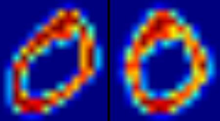
Below image shows above deskew function applied to an image of zero. Left image is the original image and right image is the deskewed image.
image
Next we have to find the HOG Descriptor of each cell. For that, we find Sobel derivatives of each cell in X and Y direction. Then find their magnitude and direction of gradient at each pixel. This gradient is quantized to 16 integer values. Divide this image to four sub-squares. For each sub-square, calculate the histogram of direction (16 bins) weighted with their magnitude. So each sub-square gives you a vector containing 16 values. Four such vectors (of four sub-squares) together gives us a feature vector containing 64 values. This is the feature vector we use to train our data.
2 gx = cv2.Sobel(img, cv2.CV_32F, 1, 0)
3 gy = cv2.Sobel(img, cv2.CV_32F, 0, 1)
4 mag, ang = cv2.cartToPolar(gx, gy)
7 bins = np.int32(bin_n*ang/(2*np.pi))
10 bin_cells = bins[:10,:10], bins[10:,:10], bins[:10,10:], bins[10:,10:]
11 mag_cells = mag[:10,:10], mag[10:,:10], mag[:10,10:], mag[10:,10:]
12 hists = [np.bincount(b.ravel(), m.ravel(), bin_n)
for b, m
in zip(bin_cells, mag_cells)]
13 hist = np.hstack(hists)
Finally, as in the previous case, we start by splitting our big dataset into individual cells. For every digit, 250 cells are reserved for training data and remaining 250 data is reserved for testing. Full code is given below:
7 svm_params = dict( kernel_type = cv2.SVM_LINEAR,
8 svm_type = cv2.SVM_C_SVC,
11 affine_flags = cv2.WARP_INVERSE_MAP|cv2.INTER_LINEAR
15 if abs(m[
'mu02']) < 1e-2:
17 skew = m[
'mu11']/m[
'mu02']
18 M = np.float32([[1, skew, -0.5*SZ*skew], [0, 1, 0]])
19 img = cv2.warpAffine(img,M,(SZ, SZ),flags=affine_flags)
23 gx = cv2.Sobel(img, cv2.CV_32F, 1, 0)
24 gy = cv2.Sobel(img, cv2.CV_32F, 0, 1)
25 mag, ang = cv2.cartToPolar(gx, gy)
26 bins = np.int32(bin_n*ang/(2*np.pi))
27 bin_cells = bins[:10,:10], bins[10:,:10], bins[:10,10:], bins[10:,10:]
28 mag_cells = mag[:10,:10], mag[10:,:10], mag[:10,10:], mag[10:,10:]
29 hists = [np.bincount(b.ravel(), m.ravel(), bin_n)
for b, m
in zip(bin_cells, mag_cells)]
30 hist = np.hstack(hists)
33 img = cv2.imread(
'digits.png',0)
35 cells = [np.hsplit(row,100)
for row
in np.vsplit(img,50)]
38 train_cells = [ i[:50]
for i
in cells ]
39 test_cells = [ i[50:]
for i
in cells]
43 deskewed = [map(deskew,row)
for row
in train_cells]
44 hogdata = [map(hog,row)
for row
in deskewed]
45 trainData = np.float32(hogdata).reshape(-1,64)
46 responses = np.float32(np.repeat(np.arange(10),250)[:,np.newaxis])
49 svm.train(trainData,responses, params=svm_params)
50 svm.save(
'svm_data.dat')
54 deskewed = [map(deskew,row)
for row
in test_cells]
55 hogdata = [map(hog,row)
for row
in deskewed]
56 testData = np.float32(hogdata).reshape(-1,bin_n*4)
57 result = svm.predict_all(testData)
60 mask = result==responses
61 correct = np.count_nonzero(mask)
62 print correct*100.0/result.size
This particular technique gave me nearly 94% accuracy. You can try different values for various parameters of SVM to check if higher accuracy is possible. Or you can read technical papers on this area and try to implement them.
Additional Resources
- Histograms of Oriented Gradients Video
Exercises
- OpenCV samples contain digits.py which applies a slight improvement of the above method to get improved result. It also contains the reference. Check it and understand it.
 1.8.9.1

