Relevant to Blender v2.31
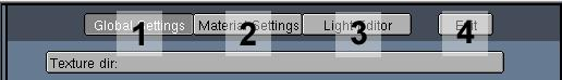
The functions of Yable have been divided in three main screens, accessible by pressing the three upper buttons that you can see in Figure 29.2, “Yable header Buttons.”.
Once we have created a Blender scene, with objects, materials and lights, we can load and start the script, possibly splitting the main 3D Viewport in two, and turning one of the two halves into a Text Window. This way we will be able to see at the same time the scene and Yable GUI.
The Yable Workflow is as follows:
Select an object of the scene;
Go to the Material or Light part of the interface, depending on what you are defining, and press the
Get Selectedbutton. This way Yable retrieves the settings for the object (if any);Edit the attributes. These are completely independent from those of Blender!
Press the
Assignbutton to assign the parameters you entered to the object. Don't forget this step! A buttonAssign Allcan be used to assign the data to all selected objects.
This part of the GUI allows us to access the functions of general scene settings Figure 29.3, “Yable headerGeneral Setting Buttons.”.
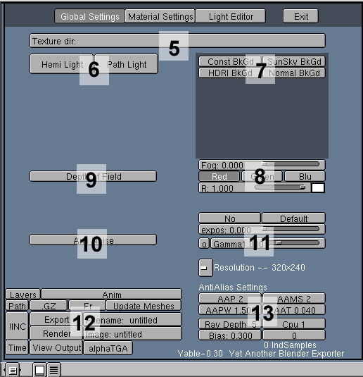
Texture path (Figure 29.3, “Yable headerGeneral Setting Buttons.”#5) - The path of the texture can be redefined anytime.
Global Illumination (Figure 29.3, “Yable headerGeneral Setting Buttons.”#6) - Adds to the scene the global illumination, that is the simulation of the diffused light, originated in nature as an effect of the infinite mutual reflections and diffusions between the objects. Its effect is added to that any possible direct lights.
Path light and Hemi light are finalized to yield of the same effect, but using different algorithms that have advantages and disadvantages, for the description of which we send back to the specific YafRay Chapter.
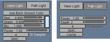
Figure 29.4, “Yable Global Illumination settings.” shows the various options for Hemi or Path light. In the former case we can set up the colour using the
Red,GreenandBlueNumButton, or take the color from the background with the buttonUse Backgroundcolor. It is possible to use this last feature when we use backgrounds based on images, even if theUse BackgroundButton disappears by setting all the three RGB slider to 0.In the Path Light case, on the other hand, the background image is used by default. Another difference between hemi and path light is the
Depthparameter, that is referred to the number of bounces to be considered in the calculation of the exchange of reflections between the objects. To get a minimum of radiosity effect it is necessary to have at least two light interchanges.Since the Path Light computation is rather complex a Cache option is provided, allowing to optimize and diminish the rendering times. It basically acts as a pre-process used to determine the zones of the image that need more samplings; as an example on a great flat surface we can presume that the diffuse lighting is quite uniform, and therefore we can carry out less calculations.
Parameters shared by both the global lights are the Power, the QMC, and the Samples. The Power indicates the power of the luminous emission, while the Samples indicates the accuracy of the sampling during the rendering: high values improve the clearness of the light (the hemi light have the tendency to become grainy) but this increase vary much the times required for calculation. QMC refers to the use of the Quasi MonteCarlo method for the determination of the zones to compute: it is based on sequences of quasi random numbers, and accelerates the rendering, even if, sometimes, it generate granular pattern of the image.
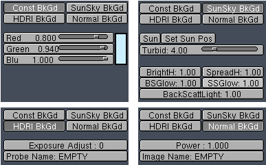
Background (Figure 29.3, “Yable headerGeneral Setting Buttons.”#7) - There are four options. Depending on the choice made some additional buttons appear, almost all are of immediate understanding (Figure 29.5, “Background settings.”).
The
Const BkGd, is the easier to use (Figure 29.5, “Background settings.” top left): it is an homogenous colour defined by its RGB values.The
Normal BkGd(Figure 29.5, “Background settings.” bottom right) allows us to use an image (the last version of YafRay supports JPG and TGA); the only parameter is thePower, that indicates the brilliance of the image.The
HDRI BkGd(Figure 29.5, “Background settings.” bottom left) is, perhaps, the one allowing for the maximum realism. The HDR (High Dynamic Range) Images, by storing pixel colours as floating point numbers contain much more data than other formats. Moreover, they are usually available as probes, that is as full 360 horizontal, 180 vertical backgrounds. After the we have obtained the appropriate images, is necessary to put them in the same folder as the textures, to write the name in theProbe Namebutton, and to set up the exposure that we want to use (positive means brighter).Finally the
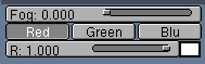
SunSky BkGd(Figure 29.5, “Background settings.” top right) uses a sophisticated algorithm for the simulation of the conditions of Sun light. The position of the sun can be set by selecting an object in the Blender scene (usually an empty) and pressing theSet Sun Posbutton and confirming. It is important to note that the dimension of the sun will depend also from the distance between the chosen object and the camera. A particularly important parameter for the construction of the scene isTurbid, that allows us to regulate the value of the density of the atmospheric layers that envelop the planet: dense layers let to go through only determined wavelengths of the solar light, hence it changes both the color and the power of the light. The other buttons control the halo and the spread of the beams. The SunSky background, if used with Path Light or Hemi Light, is able to emit light in extremely realistic ways. In the case in which we don't want to use Global Illumination we can press the Sun button and Yable will add a Sun type light in the exported scene, that will simulate, more roughly but faster, the effect of the solar light.Fog (Figure 29.3, “Yable headerGeneral Setting Buttons.”#8) - With the Fog slider we choose the amount of fog present in the scene (zero by default), while the color is chosen by selecting one of the three
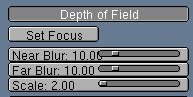
Red,GreenandBluebutton and by using the single Num Button below them (Figure 29.6, “Fog Settings.”).Depth of field (Figure 29.3, “Yable headerGeneral Setting Buttons.”#9) - This is required to mimic a real camera's focal blur. This is a feature that YafRay will render in much shorter times than other rendering engines, as it is performed as a post-processing operation - however, this means that it has some shortcomings in the precise accounting of reflections.
The regulation is made by selecting an object whichever in the scene of Blender and pressing the button
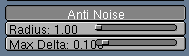
Set Focus(Figure 29.7, “Depth of Field Settings.”). The point chosen in this way will be perfectly sharp. With the others two Num Buttons we can regulate the amplitude of the field depth:Near Blurinfluences on how much will the objects that are between the camera and the point of focus be blurred, whileFar Bluraffects the objects further than the focus from the camera.Anti-noise Filter (Figure 29.3, “Yable headerGeneral Setting Buttons.”#10) - This too is a filter applied as post processing. It works in an iterative manner by taking some points within of a circular area and assign the same color if their colours differ more than a given threshold.
The amplitude of the circular area is determined by the
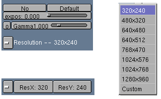
Radiusparameter (Figure 29.8, “Anti Noise Filter Settings.”), while the threshold is given byMax Delta. This is a very useful filter, but to use with care, because it has also a blurring effect that might compromise the quality of the result. Higher values of the delta tend to unify all.Gamma correction, exposure, resolution (Figure 29.3, “Yable headerGeneral Setting Buttons.”#11) - A simple group of buttons that allows you to set the brightness and the gamma of the complete rendering. The
NoButtons exclude completely both post-processes. TheDefaultButton that bring back theexposNum Button to the default value. TheGammaNum Button allows the regulation of the gamma (Figure 29.9, “Resolution Settings.”).The resolution Menu Button allows you to choose the dimension of the rendered image. Pressing it, we can choose between the most common formats:320x240, 480x320, 640x480, 640x512, 768x470, 1024x576, 1024x768 and 1280x960. Choosing the
Customoption, two new buttons are visualized, that allow to set up any resolution.Rendering setting (Figure 29.3, “Yable headerGeneral Setting Buttons.”#12) - This group of buttons allows you to set details of the exported file and let to launch YafRay directly from Blender (Figure 29.10, “Rendering Settings.”).
The fundamental keys are
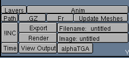
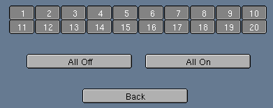
Export,Render,FilenameandImage. The last two are needed in order to choose the name that will have the XML file and the rendered image.Exportproduces only, within theYABLEROOTdirectory all the necessary XML files while, if used withRender, will also execute YafRay and will produce the final image; finally, if the button View Output is also selected, at the end of the rendering Yable will launch also the application specified inVIEWERAPP, in order to see the result. Note that you must have YafRay in your path to be able to launch it within Blender.The Layers button open a new panel for the choice of the layer to export (Figure 29.11, “Layer Selection.”).
The
Pathbutton forces the description of the scene to be exported using separate files (one main file, and sub-files to be saved in suitable folders, subdivided by materials and meshes). The location of such files will be indicated to YafRay by with the use of a full path.To the contrary, the
!INCButton will force Yable to produce a "monolithic" file. If at the moment of the export neitherPathor!INCare used, Yable will use automatically thePathoption.Rendering problems
Sometimes, by using different files, Yable incurs in some problems and may mix the objects created in previous rendering. In such case is worthwhile to use the single file, that is surely overwritten every time, or to delete the old XMLs.
The
AnimButton forces adifferentXML file to be exported for each frame of the Blender scene. Once the frames are rendered you can compose them into an animation by using Blender's Sequence Editor. TheAnimbutton implies that theFr(frame) button is also pressed, which appends to the chosen name for XML and images files a number suffix that indicates the rendered frame. All the XMLs are saved in a separate subdirectory named as the blender file with the_MOVIEsuffix.An example
Suppose our
YABLEROOTisC:/bar/and we are working with the filerobot.blend, when we pressExport, Yable will create, first of all, a folderC:/bar/robot/; then, if we have specified thePathoption, inside this directory the main XML file (calledrobot.xml) will be created, and two folders:MaterialsandMeshes, from which YafRay, reading the paths inrobot.xml, will draw the data for the materials and objects.In the case in which we choose to use the
!INCbutton, no folders will be created withinC:/bar/robot/, but only a single filerobot.xml, that contains all data.Finally, if the
Animbutton has been utilized, another folder will be created,C:/foo/robot/robot_MOVIE/containing as many XMLrobot.001.xml,robot.002.xml,robot.003.xml,... as there are frames in the animation.Note that if the files of the animation are obtained with the
Pathoption, it will be necessary to copy theMeshesandMaterialsfolders in therobot_MOVIEfolder. If the animation does not include transformations of morphing (as an example RVK), is safe to leave de-activated the buttonUpdate Mesh. Otherwise for every exported frame every mesh of the scene will be exported too.The last three buttons are
GZ,Time, andalphaTGA: the first enable the creation of gzipped files, the second let the time employed for the rendering appear on the YafRay console and the third modifies the XML so that YafRay saves TGA images with the alpha channel.Antialiasing setting (Figure 29.3, “Yable headerGeneral Setting Buttons.”#13) -
AAPNum Button indicates the number of passes of antialiasing; putting it equal to zero indicates no antialias.AAMSadjust the number of samplings to use for every AA pass.AAPWadjust the pixel width parameter, that is the overlap of pixels; the range vary between 0 and 2, and using high values, we can obtains a better smoothness, even if sometimes too much accentuate.AATestablishes the value of threshold (AA_threshold) beyond which the pixel will be processed from the antialiasing: the value can vary between 0 (all points will be processed) and 1 (no pixel are processed). CPU indicates, if multiple CPU are present, how many should be used for rendering.
The second GUI panel contains the Material Setting. Here it is possible to assign to every object the material that will be used in the YafRay rendering. The Materials assigned with Yable and Blender materials are two different things: the script draws from the scene only some values, like the UV coordinates and the diffuse color. This latter only upon request of the user. The rest is all independent; from this point of view Yable is a sort of laboratory: it not only exports passively the scene, but it allows us to study and to apply new materials.
Once an object is selected we must press the Get Selected
Button: new buttons will appear; containing YafRay settings if the Object
already has them, or empty otherwise(Figure 29.12, “Material Buttons.”).
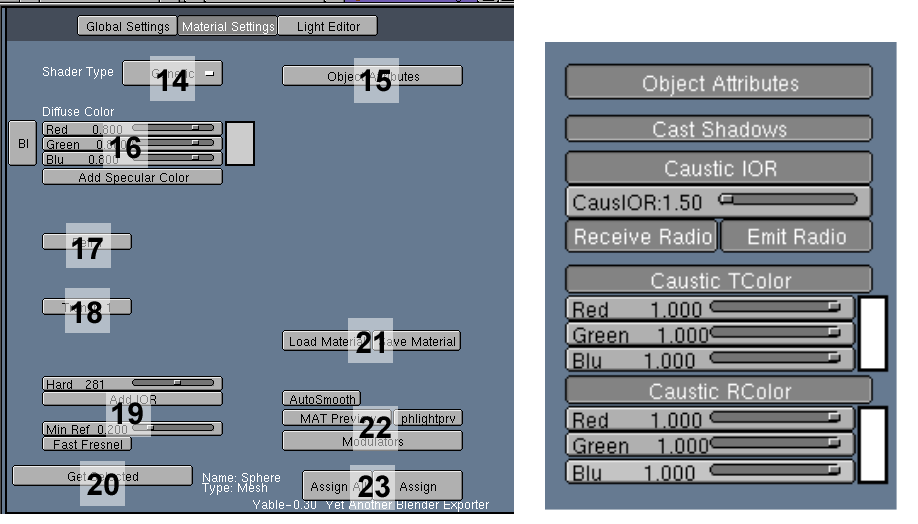
Shader Type (Figure 29.12, “Material Buttons.”#14) - This button allows you to choose the Type of Material Shader to apply.
The
Constantshader is the simplest, characterized only from theRed,GreenandBluNum Buttons.Crafteris a distinct case: it is an interface used to loading the Crafter shader, that is a stand alone program for the visual composition of materials.Genericis the more versatile material, and includes also the characteristics of the others, hence we will describe it deeply, using it like a paradigm for the general understanding.Object Attributes (Figure 29.12, “Material Buttons.”#14) - Pressing this button some new buttons appear (Figure 29.12, “Material Buttons.” on the right). They are very important characteristics, which are linked to the Object and not to the Material itself. The
Cast Shadowtoggles if the object projects shadows or not. TheCaustic IORbutton enables the calculation of the caustics for the light beams that will pass through the object; these will be deflected according to the value of the refractive index indicated fromCausIORNumButton. High IOR values produce more sharp caustics (think, as an idea, to the lens that concentrates the solar beams in a point). TheReceive Radioand theEmit Radiobuttons, if pressed, will force the object to participate to the calculation of the global illumination, receiving and re-emitting energy. TheCaustic TcolorNum Buttons allows you to specify the transmitted colour, that is the colour assumed from the light passing through the Object. TheCaustic RcolorNum Buttons, on the other hand, refers to the light reflected by the Object.Note
Note that even if we set correctly a material, it will participate to the effects of caustics and radiosity only if it is illuminated with appropriate lights, like the Path Light, or the Photon Light.
Diffuse Colour (Figure 29.12, “Material Buttons.”#16) - Is the basic color, and corresponds to the Diffuse Colour in Blender materials. The Bl button on the side is used take RGB values directly from the Blender Material. Pressing the button
Add Specular Colornew buttons appear similar to those just seen, used to set the specular color. Also in this case the meaning of this Colour is the same to that of Blender.Reflection and Transmission Colours (Figure 29.12, “Material Buttons.”#17 and #18) - It is possible to set the Reflected and Transparency colours of the material. Note that also the transparency is set using the RGB Num Buttons to define a Colour, not just a plain "alpha" value.
The Transmit parameter does not decide the degree of transparency, but only which color of the light pass through (or is blocked by) the material. To make some example, using the black colour we impose that no color passes through the material, using the red one, we would mean that the object is transparent only for the red component of the light, using the white we let all the light to pass. Pressing also the buttons
Refl2andTransm2which appears we can (and new RGB Num Buttons are created) define a different behaviour of the material at grazing light incidence.Hardness, Index of Refraction (Figure 29.12, “Material Buttons.”#19) - The
hardparameter governs the sharpness of specular highlights exactly as in Blender. The refractive indexIORis fundamental in transparent objects, and is used in order to calculate the deviation of the light beams that crosses the material. As a result of this effect, the bodies immersed in a transparent medium appears to us distorted (think to a paddle immersed in the limpid water). Table 29.1, “Sample IORs” shows some IORs of common materials:Get Selected (Figure 29.12, “Material Buttons.”#20) - The
Get Selected, to be pressed every time after you have selected the object and before starting to modify the material.Get Selected, Loading and saving the materials (Figure 29.12, “Material Buttons.”#21) - The
Load MaterialandSave Materialbuttons allows you to save material settings and to quickly call them back. A name can be given to each material.Preview of the material, autosmooth and modulators (Figure 29.12, “Material Buttons.”#22) - The
AutoSmoothButton is used to regulate the appearance of the surfaces. Pressing it an additional Num Button appears that regulated the angle under which the corner of the two faces is considered smooth, exactly as in Blender.The
Mat previewButton creates a preview of the material using a sample scene. The tga is saved in the current directory (for example, under Windows, it is saved in the folder in which the Blender executable resides.) The buttonphlightprvindicate "Photon Light Preview" and it is used to put a photonic light during the materials preview.The
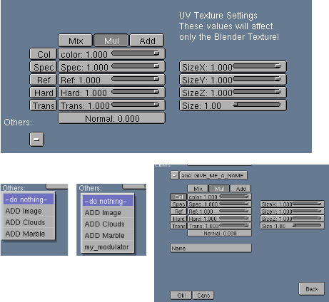
ModulatorsButton allows you to access a separate panel for the composition of advanced shaders formed by overlying layers. Every layer can be an image or a procedural texture. Obviously is possible to set the modality with which the layers must be mixed and also the percentage of transparency.The panel at the beginning refers to the default modulators, that is used automatically if the Object has UV coordinates and is mapped with an image in Blender. Unfortunately, because of a bug, these formulations are not maintained by Yable, that continues to use the default settings. However all the successive layers of modulators that are added work correctly. In order to add a new component is sufficient to click on the Others button, and to choose the kind of modulator that we want. In Figure 29.13, “Material Modulators.” we see (starting from the top left, clockwise) the main panel, the panel adding new members, the menu
Others, before and after the addiction of a new member:It is possible to add an
Imagelayer, aCloudslayer and aMarbleone. The first thing is to assign a name at the modulator created, to do this it will be sufficient to write something of meaningful in place ofGIVE_ME_A_NAME.If the Modulator is an image it is necessary to insert the name of the image itself: only the name and extension, without path, which has been defined once for all before!
The parameters refer, by default, to bump mapping, that is to the relief effect that will be given to the object: using positive values rises clearer zones and lowers darker. The various size refer to the scaling of the UV coordinates (the three X, Y, Z axis may be scaled independently, or all together) while the various buttons
Col,Spec,Ref,HardandTranshave the usual meanings and indicates which characteristic, and by how much, is modified. At the end of the settings, press theOk!button, to return to the main Material panel. At the end of the procedure the new added modulator will be in the Menu and can be selected and cancelled anytime, using the buttonDelthat appear next to theOk!CancandBackbuttons.Note
The only type of mapping supported up to now is the UV type. It follow that the object must possess these coordinates, for which we sends back to the relevant Section of this Guide. If all is correctly executed, Yable will export automatically (without the adding of an image type modulator) both the UV coordinates and the used image. About this image we must pay attention to this: Yable does not use the image loaded in the texture of Blender's materials, but the one loaded in the Image Window (that is the one on which calculations for the positioning of the UV are made). Obviously, the images must all be in the usual folder specified at the start of the script.
Clouds and Marble Modulators insertion is similar to that for the Images, except that these panels have few additional, self explanatory, specific parameters for these two types of procedural texture.
Assign (Figure 29.12, “Material Buttons.”#23) - The
Assignbutton finalizes the material and assigns it to the object. Don't forget this! The button Selected All allows you to assign the settings to more than one selected objects.Note
Saving a material and Assigning a material are two separate actions. If you assign it the Object acquires that material, if you save it, it will be available later on.
The lights setting in Yable is made with the same modality of the materials
assignation: a light is selected in Blender, Get Selected
is pressed and the characteristics that we want to to export in YafRay
are chosen and assigned definitively with Assign.
The type of light used in the scene of Blender do not have any relationship with the type of light that will be exported: the only parameters that will be surely conserved are the positional coordinates of the lamp; all the rest, included the pointing direction can be assigned independently with Yable. In Figure 29.14, “Light GUI Panel.” we have represented a point light with the buttons Diffuse and Caustic activated, so to have an example that include the greater part of the available options.
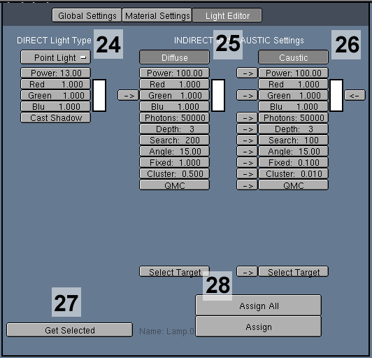
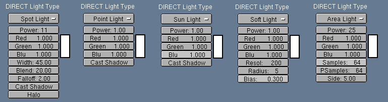
Light Types (Figure 29.12, “Material Buttons.”#24) - The menu lets us choose between various types of direct light:
Point Light,Spot Ligth,Soft light,Area LightandPhoton Light. Accordingly to the light type the options immediately beneath varies. Figure 29.15, “Direct Light Options.” shows them all.The Point light is a point source that emits light in all the directions. The power of the lamp is chosen with the
PowerNum Button, while its colour is set via RGB Num Buttons and is possible to choose if it must project or not a shadow with theCast ShadowButton.The Spot light is very similar to the Blender spot: the parameters
BlendandFalloffhave the same meaning, whileWidthrepresents the angular width of the light cone.Haloindicates the presence of the halo (volumetric light), by pressing it we add some new buttons: three Num Buttons for the Halo colour,Res= resolution of the shadow map,Density= quantity of fog contained in the halo,Blur= blur applied to shadow map,Samples= number of samplings used in the rendering.The direction of the Spot is given via a target. We must press the
Select Targetbutton, select an Object to be the target of the spot in the Blender scene and finally press theConfirmButton to complete the operation.Both the Point and the Spot light decreases following the physical law of the inverse square of the distance.
The Soft light is similar to the Pointlight, with the difference that it produces soft shadows. Shadows which appear to be too "clean" are one of the disadvantages of the raytrace engines, but this type of light, using a shadow map, safely resolves the problem. Besides the usual parameters, the
Radiusparameter, defines the width of the transition between shadow and light. TheBiasparameter controls the proximity of the shadow to the object that produces it, while theResolparameter controls the resolution of the shadow map: the higher is this parameter the better is the accuracy of the shadow.The Sun light simulates the characteristic of the solar light, it seems not to decay with increasing of the distance (it is an impression due to the enormous power of the Sun). It is, therefore, a much simple light, in which we can only set up the color, and whose intensity remains constant.
The Area light is an extended luminous source. While all those already seen emit light from a point (in reality it corresponds, as an example, to the small filament of a light bulb), the area light is produced from a whole surface. YafRay admit also quadrilateral surfaces but Yable is limited to use only squares. The specific parameters are
Samples,PsamplesandSide, they are the number of general samplings, the number of samplings in the penumbra zone, and the length of the side of the light casting square.Photon Lights (Diffuse and Caustic) (Figure 29.12, “Material Buttons.”#25 and #26) - Photonlight is a very peculiar kind of lamp: it behave in a more realistic way, referring itself to the theory of the light composed by a bundle of photons. These photons must literally be "shoot" towards the Objects, so as to calculate their behaviour when they travel through transparent bodies or are diffused by opaque ones. It is a very complex calculation, for which is not always desirable that it will be executed on all the elements of the scene; therefore we can specify it on a material to material and object by object basys via the parameters Receive and Emit.
Diffuse light: Enabling this button a Photon Light of Diffuse type will be add to the exported scene, overlapping the corresponding Direct light. The photons of this light have the capability to be reflected on diffusive surfaces. In this way calculations of the radiosity 'colour leakage' will be added in the rendering, to realize a realistic effect of Global Illumination. This can be done also via Path Light, but a carefully tuned Photon Light is much faster.
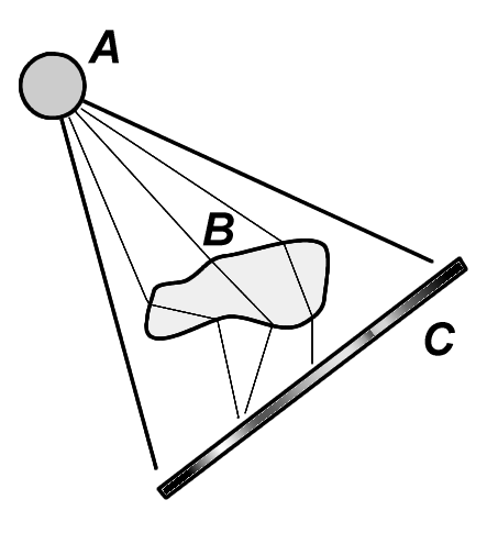
Caustic light: Caustic are concentrations of light caused from the refraction of the transparent objects. The Photon Light of Caustic type allows you to account for this phenomenon correctly. Before going ahead, it is necessary to say that if targeted to objects with inadequate material, this light does not generate any effect. In fact the scene, to have caustics, must contain a source light A, an opaque object C receiving the caustics and a transparent object B placed between these two generating the caustics (Figure 29.16, “Caustics setup.”).
A must be a caustic photonlight;
B must have a Material able to produce Caustics (exhibiting at leastassigning at least Caustic IOR and Caustic Tcolor);
C must have a Material able to receive the radiosity effects (for this the default material could be good, because this material export a simple shader that, without specify the received and emitted values of radiosity leave the choice to YafRay, that usually hold this values activated. If, indeed, a generic material is used, we must remember to activate the
Reiceve RadioToggle Button).
The Photon Light of Caustic and Diffuse type have the same parameters. The arrows button is used to impose the same value to more than one variables (for example the same color ).
The
Photonsbutton set the number of photons that will be shot from the lamp, in common scene a few thousands of photons is enough but, to obtain a better results in terms of quality is recommended to set 50000 photons or more. TheDepthbutton defines the number of bounces/transmissions the photons can do before YafRay ray tracing stops to handle it, and it is a particularly important data, mostly in the calculation of the Global illumination. 3 is a good value for acceptable results.Searchindicates the numbers of photons that can be used to illuminate a single point of the Object surface, higher values is used to take in consideration also zones that receive few photons, with a shaded effect of illumination, while low value is used to give light only to the points really hit by photons completely, with more definite and "hard" boundaries.Angleis the angle of the projection cone with which the photon are shot: high values are used to cover a wide area, but with power fading when we depart from the center.Fixedis the abbreviation of fixedradius, and represent the radius in which the number of photons defined bySearchmust fall in order to consider the point of the surface illuminated.clusteris the smallest portion of lit surface able to contain a photon. The higher is this number the larger is the width of the cluster and, consequently, the less defined is the illumination effect.QMCis, again, the quasi-MonteCarlo method.