Appendix B: Using the Driverless AI Python Client¶

This section describes how to run Driverless AI using the Python client.

Notes:

This is an early release of the Driverless AI Python client.
Python 3.6 is the only supported version.
You must install the h2oai_client wheel to your local Python. This is available from the PY_CLIENT link in the top menu of the UI.

Running an Experiment¶

After the h2oai_client wheel is installed, import the required modules and log in.

import h2oai_client
import numpy as np
import pandas as pd
import requests
import math
from h2oai_client import Client, ModelParameters, InterpretParameters

address = 'http://ip_where_driverless_is_running:12345'
username = 'username'
password = 'password'
h2oai = Client(address = address, username = username, password = password)
# Be sure to use the same credentials that you use when signing in through the GUI

Upload training, testing, and validation datasets from the Driverless AI /data folder. The validation and testing dataset are optional. This example shows how to add a validation dataset, but the experiment will only specify training and testing datasets.

train_path = '/data/CreditCard/CreditCard-train.csv'
test_path = '/data/CreditCard/CreditCard-test.csv'
valid_path = '/data/CreditCard/CreditCard-valid.csv'

train = h2oai.create_dataset_sync(train_path)
test = h2oai.create_dataset_sync(test_path)
valid = h2oai.create_dataset_sync(valid_path)

Set experiment parameters:

The next step is to set parameters for the experiment. Some of the parameters include:
- Target Column: The column we are trying to predict.
- Dropped Columns: The columns we do not want to use as predictors such as ID columns, columns with data leakage, etc.
- Weight Column: The column that indicates the per row observation weights. If “None”, each row will have an observation weight of 1.
- Fold Column: The column that indicates the fold. If “None”, the folds will be determined by Driverless AI.
- Time Column: The column that provides a time order, if applicable. If “AUTO”, Driverless AI will auto-detect a potential time order. If “OFF”, auto-detection is disabled.
For this example, we will be predicting default payment next month. We can set the parameters by hand or let Driverless AI infer the parameters and override any we disagree with. In this case, we will let Driverless AI suggest the best parameters for our experiment.

# let Driverless suggest parameters for experiment
target="default payment next month"
params = h2oai.get_experiment_tuning_suggestion(dataset_key = train.key, target_col = target)

params.dump()
{'accuracy': 7,
 'cols_to_drop': [],
 'dataset_key': 'corulege',
 'enable_gpus': True,
 'fold_col': '',
 'interpretability': 7,
 'is_classification': True,
 'scorer': '',
 'seed': False,
 'target_col': 'default payment next month',
 'testset_key': '',
 'time': 3,
 'time_col': '',
 'validset_key': '',
 'weight_col': ''}

Driverless AI has found that the best parameters are to set accuracy = 7, time = 3, and interpretability = 7. We will add our test data to the parameters, set the scorer to AUC, and add a seed to make the experiment reproducible.

params.testset_key = test.key
params.scorer = "AUC"
params.seed = 1234

Launch the experiment to run feature engineering and final model training. In addition to the settings previously defined, be sure to also specify the imported training dataset. Adding a test dataset and a validation dataset is optional. This example will not use a validation dataset.

experiment = h2oai.start_experiment_sync(params)

Examine the final model score for the valildation and test datasets. When feature engineering is complete, an ensemble model can be built depending on the accuracy setting. The experiment object also contains the score on the validation and test data for this ensemble model.

print("Final Model Score on Validation Data: " + str(round(experiment.valid_score, 3)))
print("Final Model Score on Test Data: " + str(round(experiment.test_score, 3)))

Final Model Score on Validation Data: 0.779
Final Model Score on Test Data: 0.802

The experiment object also contains the scores calculated for each iteration on bootstrapped samples on the validation data. In the iteration graph in the UI, we can see the mean performance for the best model (yellow dot) and +/- 1 standard deviation of the best model performance (yellow bar).

This information is saved in the experiment object.

import matplotlib.pyplot as plt

iterations = list(map(lambda iteration: iteration.iteration, experiment.iteration_data))
scores_mean = list(map(lambda iteration: iteration.score_mean, experiment.iteration_data))
scores_sd = list(map(lambda iteration: iteration.score_sd, experiment.iteration_data))

plt.figure()
plt.errorbar(iterations, scores_mean, yerr=scores_sd, color = "y",
           ecolor='yellow', fmt = '--o', elinewidth = 4, alpha = 0.5)
plt.xlabel("Iteration")
plt.ylabel(scorer_str)
plt.show();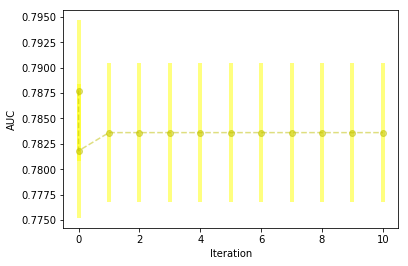

We will show an example of downloading the test predictions below. Note that equivalent commands can also be run for downloading the train (holdout) predictions.

h2oai.download(src_path=experiment.test_predictions_path, dest_dir=".")
'./test_preds.csv'

test_preds = pd.read_csv("./test_preds.csv")
test_preds.head()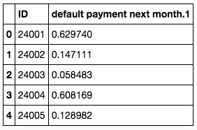
We can also download and examine the summary of the experiment and feature importance for the final model.
# Download Summary
import subprocess
summary_path = h2oai.download(src_path=experiment.summary_path, dest_dir=".")
dir_path = "./h2oai_experiment_summary_" + experiment.key
subprocess.call(['unzip', '-o', summary_path, '-d', dir_path], shell=False)
The table below shows the feature name, its relative importance, and a description. Some features will be engineered by Driverless AI and some can be the original feature.
# View Features
features = pd.read_table(dir_path + "/features.txt", sep=',', skipinitialspace=True)
features.head(n = 10)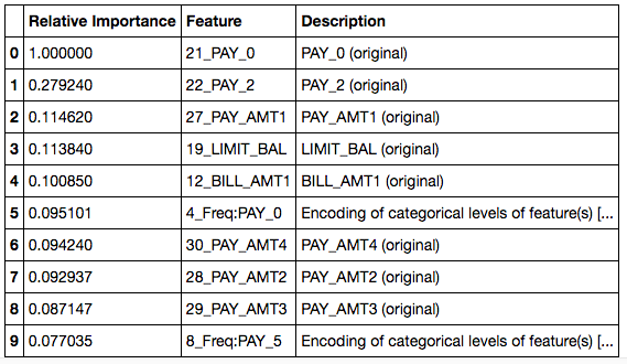

Access an Experiment Object that was Run through the Web UI¶

It is also possible to use the Python API to examine an experiment that was started through the Web UI using the experiment key.

You can get a pointer to the experiment by referencing the experiment key in the Web UI.

# Get a list of experiments
experiment_list = list(map(lambda x: x.key, h2oai.list_models(offset=0, limit=100)))
experiment_list
['fapudage', 'cunegacu', 'hamasida']

# Get pointer to experiment
experiment = h2oai.get_model_job(experiment_list[0]).entity

Score on New Data¶

You can use the Python API to score on new data. This is equivalent to the SCORE ON ANOTHER DATASET button in the Web UI. The example below scores on the test data and then downloads the predictions.

Pass in any dataset that has the same columns as the original training set. If you passed a test set during the H2OAI model building step, the predictions already exist. Its path can be found with experiment.test_predictions_path.

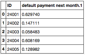
The following shows the predicted probability of default for each record in the test.

prediction = h2oai.make_prediction_sync(experiment.key, test_path, output_margin = False, pred_contribs = False)
pred_path = h2oai.download(prediction.predictions_csv_path, '.')
pred_table = pd.read_csv(pred_path)
pred_table.head()

We can also get the contribution each feature had to the final prediction by setting pred_contribs = True. This will give us an idea of how each feature effects the predictions.

prediction_contributions = h2oai.make_prediction_sync(experiment.key, test_path, output_margin = False, pred_contribs = True)
pred_contributions_path = h2oai.download(prediction_contributions.predictions_csv_path, '.')
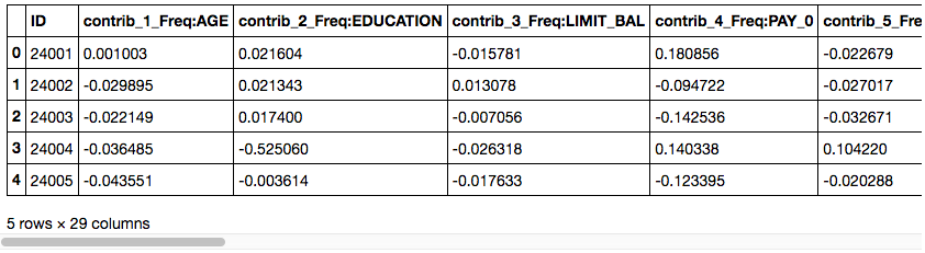
pred_contributions_table = pd.read_csv(pred_contributions_path)
pred_contributions_table.head()

We will examine the contributions for our first record more closely.

contrib = pd.DataFrame(pred_contributions_table.iloc[0][1:], columns = ["contribution"])
contrib["abs_contribution"] = contrib.contribution.abs()
contrib.sort_values(by="abs_contribution", ascending=False)[["contribution"]].head()

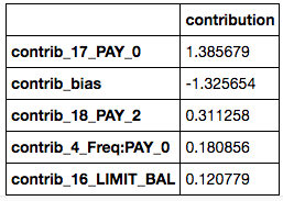
This customer’s PAY_0 value had the greatest impact on their prediction. Because the contribution is positive, we know that it increases the prediction that they will default.

Run Model Interpretation¶

Once we have completed an experiment, we can interpret our H2OAI model. Model Interpretability is used to provide model transparency and explanations. You can run model interpretation on raw data and on external model predictions.

Run Model Interpretation on Raw Data¶

We can run the model interpretation in the Python client as shown below. By setting the parameter, use_raw_features to True, we are interpreting the model using only the raw features in the data. This will not use the engineered features we saw in our final model’s features to explain the data. If you set use_raw_features to False, the model will be interpreted using the features used in the final model (raw and engineered).

Note that you can also specify the number of cross-validation folds to use in K-LIME. This defaults to 0.

mli_experiment = h2oai.run_interpretation_sync(InterpretParameters
                     (dai_model_key=experiment.key,
                      dataset_key=train.key,
                      target_col=target,
                      prediction_col = '',
                      use_raw_features=True, # show interpretation based on the original columns
                      klime_cluster_col='',
                      nfolds = 0 # number of folds used for k-lime
                     ))

You can also see the list of interpretations using the Python client.

# Get list of interpretations
mli_list = list(map(lambda x: x.key, h2oai.list_interpretations(offset=0, limit=100)))
mli_list

['wekature', 'bawamoci']

Run Model Interpretation on External Model Predictions¶

Model Interpretation does not need to be run on a Driverless AI experiment. You can train an external model and run Model Interpretability on the predictions. In this next section, we will walk through the steps to interpret an external model.

Train External Model¶

We will begin by training a model with scikit-learn. Our end goal is to use Driverless AI to interpret the predictions made by our scikit-learn model.

# Dataset must be located where python client is running
train_pd = pd.read_csv(train_path)

from sklearn.ensemble import GradientBoostingClassifier

predictors = list(set(train_pd.columns) - set([target]))

gbm_model = GradientBoostingClassifier(random_state=10)
gbm_model.fit(train_pd[predictors], train_pd[target])
GradientBoostingClassifier(criterion='friedman_mse', init=None,
              learning_rate=0.1, loss='deviance', max_depth=3,
              max_features=None, max_leaf_nodes=None,
              min_impurity_decrease=0.0, min_impurity_split=None,
              min_samples_leaf=1, min_samples_split=2,
              min_weight_fraction_leaf=0.0, n_estimators=100,
              presort='auto', random_state=10, subsample=1.0, verbose=0,
              warm_start=False)

predictions = gbm_model.predict_proba(train_pd[predictors])
predictions[0:5]
array([[ 0.38111179,  0.61888821],
       [ 0.44396186,  0.55603814],
       [ 0.91738328,  0.08261672],
       [ 0.88780536,  0.11219464],
       [ 0.80028008,  0.19971992]])

Interpret on External Predictions¶

Now that we have the predictions from our scikit-learn GBM model, we can call Driverless AI’s h2o_ai.run_interpretation_sync to create the interpretation screen.

train_gbm_path = "./CreditCard-train-gbm_pred.csv"
predictions = pd.concat([train_pd, pd.DataFrame(predictions[:, 1], columns = ["p1"])], axis = 1)
predictions.to_csv(path_or_buf=train_gbm_path, index = False)

train_gbm_pred = h2oai.upload_dataset(train_gbm_path)

mli_external = h2oai.run_interpretation_sync(
    InterpretParameters(dai_model_key="",
                        dataset_key=train_gbm_pred.strip("\""),
                        target_col=target,
                        prediction_col = "p1",
                        use_raw_features=True, # not relevant since we are interpreting our external model
                        klime_cluster_col='',
                        nfolds = 0 # number of folds used for k-lime
                       ))