New in v0.46.

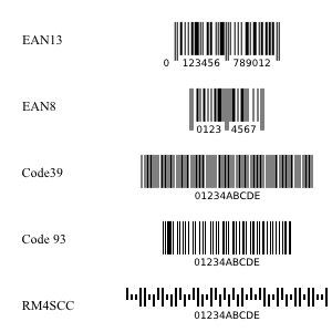
This effect generates barcodes. The types of codes that can be generated are:

Examples of barcodes.

Updated in v0.46 with plotting using polar coordinates.

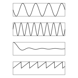
Plot a function versus x (horizontal axis). To use, first draw a rectangle to define the width of the x-axis and the height of the ±1 lines of the y-axis. Then select the effect. In the pop-up window, enter the x and y ranges. Checking the Multiply x-range by 2π box changes the x-axis to represent units of 2π, useful for plotting periodic functions. You can either have the routine calculate the first derivative of the function numerically or supply the first derivative yourself.

The function is plotted in the SVG coordinate system, which has the y-axis upside down. The effect inserts a minus sign automatically to correct for this.

All Python math functions are allowed (as long as they return a single value) including Python random number functions. The Help Tab has a list of some of the available functions.

From top to bottom: -sin(x) with four periods. sin(x) with eight periods. sin(x)/(x+0.000001) with four periods; the first point has been deleted as the first derivative estimate is off. x-floor(x) with one period. The gray boxes show the location and size of the original rectangles.

As of v0.46 plotting can be done using polar coordinates. For users of earlier versions, the necessary files can be found on the book's website.

When the Plot using Polar Coordinates option is selected, the x-range is set to −1 at the left of the rectangle and +1 at the right side. The x values entered in the effect's dialog are used for the angle domain (in radians). The Isotropic scaling parameter is ignored. Calculate first derivative numerically must also be selected.

From left to right, all with Multiply x-range by 2*pi selected and y range from -1.0 to 1.0: exp(-0.185*x), logarithmic spiral, found often in nature, x range from -5 to 0. sin(5*x) with range from 0 to 1. sin(4.0/5.0*x), range from 0 to 5. 1+0.2*sin(3*x)*sin(100.0/7.0*x), x range from 0 to 7. The gray boxes show the location and size of the original rectangles.

Note that depending on the version, Python may return an integer if you divide two integers: thus, 4/5 = 0, while 4.0/5.0 = 0.8.

New in v0.46. For users of earlier versions, the necessary files can be found on the book's website.

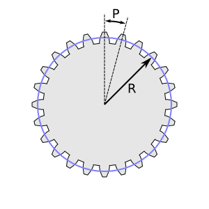
Draw a realistic mechanical gear. Three parameters must be given: the Number of teeth, the Circular pitch (the tangential distance between successive teeth), and the Pressure angle. Common values for Pressure angle are: 14.5, 20, and 25 degrees. The radius of the “Pitch Circle” is equal to N×P/2π, where “N” is the number of teeth and “P” is the Circular Pitch.

The gear is created around the SVG origin and then placed inside a Group. The Group is then translated so that the center of the gear is at the center of the visible canvas. This make animating the gear easier as the rotation is then independent of the displacement. An animated clock using these gears can be found on the book's website.

A gear with 24 teeth. The Pitch Circle is shown in blue. The Circular pitch is the distance along the Pitch Circle between the two dotted lines. “R” is the radius of the Pitch Circle.

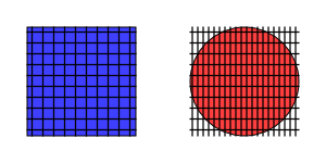
This effect fills the bounding box of an object with a grid. The grid spacing and offset can be independently set in the horizontal and vertical directions. The grid line width can also be set.

Top: Left: Grid with default settings. Bottom: Right: Grid with different horizontal and vertical spacings. Note that it is the bounding box that is filled by the grid, not the object's area. To fill an area, use a pattern or use a clip path.

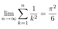
This effect turns a LaTeX string into a path. The string is typed into a dialog box. The effect requires that ghostscript, LaTeX, and Pstoedit to be installed and in the execution path. Pstoedit must include the GNU libplot SVG driver or the shareware SVG plug-in, available for Windows at the Pstoedit website. The resulting formula is rendered as a path.

An example of a formula generated by the LaTeX Formula effect.

An alternative script for Linux using Skencil for the conversion to SVG (avoiding the need for Pstoedit with SVG support) is available at the book's website: http://tavmjong.free.fr/INKSCAPE/.

Draws Lindenmayer System structures, developed by Aristid Lindenmayer while studying yeast and fungi growth patterns. It is beyond the scope of this manual to discuss these structures. Just one comment: The Step parameter controls the scale of the generated path.

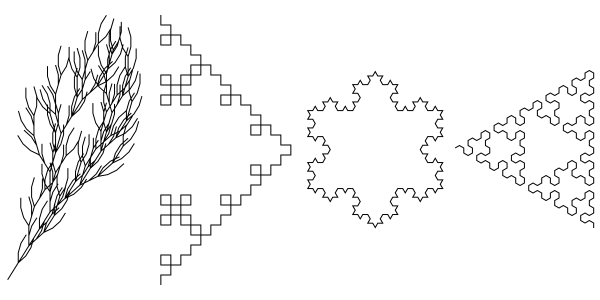
Lindenmayer Systems: From left to right:

Default inputs.

Variant of the Koch curve. Inputs: Order 3, Angles 90, Axiom F, Rules F=F+F-F-F+F.

Koch's Snowflake: Inputs: Order 3, Angles 60, Axiom F++F++F, Rules F=F-F++F-F.

Sierpinski triangles. Inputs: Order 5, Angles 60, Axiom A, Rules A=B-A-B;B=A+B+A.

The rules can be very complex. See the Lindenmayer screenshot for more information.

Draw a random tree made of straight-line segments. This is a classic from Turtle Geometry. This implementation is rather limited.

Trees drawn with the Random Tree extension.

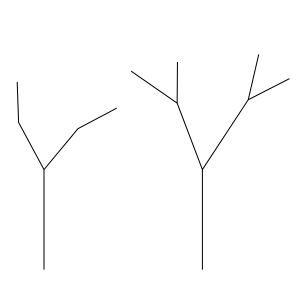
New in v0.46. For users of earlier versions, the necessary files can be found on the book's website.

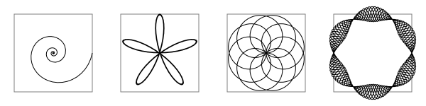
Draw a Spirograph; i.e., an epitrochoid or hypotrochoid curve. Several parameters need to be given: “R”, the Ring Radius; “r”, the Gear Radius; and “d”, the Pen Radius. In addition, one must choose if the Gear travels Inside or Outside the Ring. One can also set the Rotation angle (the angle of the starting point relative to the center) and the Quality (roughly, the number of nodes per loop).

A Spirograph drawing (Epitrochoid). R = 48, r = 36, d = 30.

A Spirograph drawing (Hypotrochoid). R = 120, r = 36, d = 30.

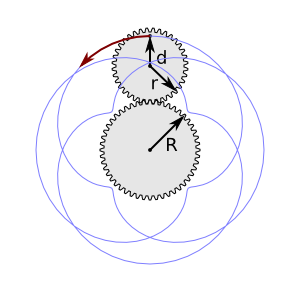
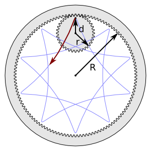
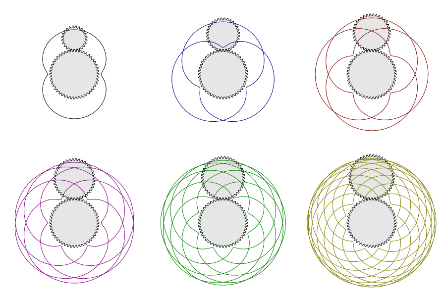
The ratio of “r” to “R” determines the structure of the curve. Take, for example, an “r” of 36 and an “R” of 48. The ratio reduced to its simplest form is 3/4. This indicates that the Gear will make a total of four “loops” as it circles the Ring three times. Simple ratios make simple curves. If you use an Even-odd fill rule, the center of the figure will be unfilled if the denominator is even.

Unlike the case with a real Spirograph that utilizes plastic gears, it is possible to specify values of “r” and “R” that don't form a rational number ratio. In this case, the curve never closes on itself and is of infinite length. To avoid such infinities, the effect limits the number of nodes to 1000. If the numerator or denominator of the ratio in the simplest form is a large integer, the Spirograph may run out of nodes. In this case, decreasing the Quality may help.

Spirographs (Epitrochoids). R = 48 for all. From left to right, top to bottom: r = 24, 32, 36, 40, 42, and 44; giving ratios of r/R of 1/2, 2/3, 3/4, 5/6, 7/8, and 11/12 respectively. In all cases d = r − 6.

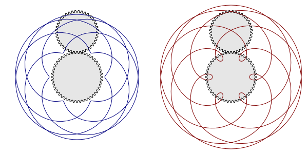
Also, unlike a “real” Spirograph, the Spirograph effect allows “d” to be greater than “r”. This results in small loops along the Ring.

Spirographs with d < r (left) and d > r (right).