8 Chart Parsing and Probabilistic Parsing
8.1 Introduction
Chapter 7 started with an introduction to constituent structure in English, showing how words in a sentence group together in predictable ways. We showed how to describe this structure using syntactic tree diagrams, and observed that it is sometimes desirable to assign more than one such tree to a given string. In this case, we said that the string was structurally ambiguous; and example was old men and women.
Treebanks are language resources in which the syntactic structure of a corpus of sentences has been annotated, usually by hand. However, we would also like to be able to produce trees algorithmically. A context-free phrase structure grammar (CFG) is a formal model for describing whether a given string can be assigned a particular constituent structure. Given a set of syntactic categories, the CFG uses a set of productions to say how a phrase of some category A can be analyzed into a sequence of smaller parts α1 ... αn. But a grammar is a static description of a set of strings; it does not tell us what sequence of steps we need to take to build a constituent structure for a string. For this, we need to use a parsing algorithm. We presented two such algorithms: Top-Down Recursive Descent (7.5.1) and Bottom-Up Shift-Reduce (7.5.2). As we pointed out, both parsing approaches suffer from important shortcomings. The Recursive Descent parser cannot handle left-recursive productions (e.g., productions such as np → np pp), and blindly expands categories top-down without checking whether they are compatible with the input string. The Shift-Reduce parser is not guaranteed to find a valid parse for the input even if one exists, and builds substructure without checking whether it is globally consistent with the grammar. As we will describe further below, the Recursive Descent parser is also inefficient in its search for parses.
So, parsing builds trees over sentences, according to a phrase structure grammar. Now, all the examples we gave in Chapter 7 only involved toy grammars containing a handful of productions. What happens if we try to scale up this approach to deal with realistic corpora of language? Unfortunately, as the coverage of the grammar increases and the length of the input sentences grows, the number of parse trees grows rapidly. In fact, it grows at an astronomical rate.
Let's explore this issue with the help of a simple example. The word fish is both a noun and a verb. We can make up the sentence fish fish fish, meaning fish like to fish for other fish. (Try this with police if you prefer something more sensible.) Here is a toy grammar for the "fish" sentences.
|
Note
Remember that our program samples assume you begin your interactive session or your program with: import nltk, re, pprint
Now we can try parsing a longer sentence, fish fish fish fish fish, which amongst other things, means 'fish that other fish fish are in the habit of fishing fish themselves'. We use the NLTK chart parser, which is presented later on in this chapter. This sentence has two readings.
|
As the length of this sentence goes up (3, 5, 7, ...) we get the following numbers of parse trees: 1; 2; 5; 14; 42; 132; 429; 1,430; 4,862; 16,796; 58,786; 208,012; ... (These are the Catalan numbers, which we saw in an exercise in Section 5.5). The last of these is for a sentence of length 23, the average length of sentences in the WSJ section of Penn Treebank. For a sentence of length 50 there would be over 1012 parses, and this is only half the length of the Piglet sentence (Section (4)), which young children process effortlessly. No practical NLP system could construct all millions of trees for a sentence and choose the appropriate one in the context. It's clear that humans don't do this either!
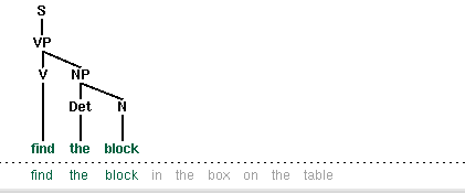
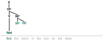
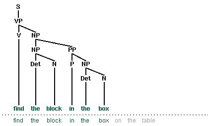
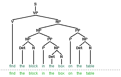
Note that the problem is not with our choice of example. [Church & Patil, 1982] point out that the syntactic ambiguity of pp attachment in sentences like (1) also grows in proportion to the Catalan numbers.
| (1) | Put the block in the box on the table. |
So much for structural ambiguity; what about lexical ambiguity? As soon as we try to construct a broad-coverage grammar, we are forced to make lexical entries highly ambiguous for their part of speech. In a toy grammar, a is only a determiner, dog is only a noun, and runs is only a verb. However, in a broad-coverage grammar, a is also a noun (e.g. part a), dog is also a verb (meaning to follow closely), and runs is also a noun (e.g. ski runs). In fact, all words can be referred to by name: e.g. the verb 'ate' is spelled with three letters; in speech we do not need to supply quotation marks. Furthermore, it is possible to verb most nouns. Thus a parser for a broad-coverage grammar will be overwhelmed with ambiguity. Even complete gibberish will often have a reading, e.g. the a are of I. As [Klavans & Resnik}, 1996] has pointed out, this is not word salad but a grammatical noun phrase, in which are is a noun meaning a hundredth of a hectare (or 100 sq m), and a and I are nouns designating coordinates, as shown in Figure 8.1.
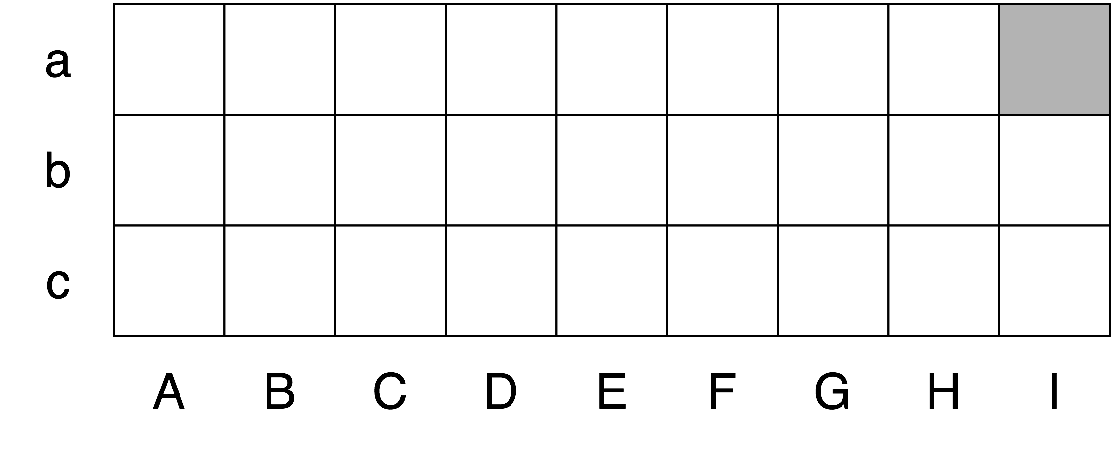
Figure 8.1: The a are of I
Even though this phrase is unlikely, it is still grammatical and a a broad-coverage parser should be able to construct a parse tree for it. Similarly, sentences that seem to be unambiguous, such as John saw Mary, turn out to have other readings we would not have anticipated (as Abney explains). This ambiguity is unavoidable, and leads to horrendous inefficiency in parsing seemingly innocuous sentences.
Let's look more closely at this issue of efficiency. The top-down recursive-descent parser presented in Chapter 7 can be very inefficient, since it often builds and discards the same sub-structure many times over. We see this in Figure 8.1, where a phrase the block is identified as a noun phrase several times, and where this information is discarded each time we backtrack.
Note
You should try the recursive-descent parser demo if you haven't already: nltk.draw.srparser.demo()
|
|
|
|
In this chapter, we will present two independent methods for dealing with ambiguity. The first is chart parsing, which uses the algorithmic technique of dynamic programming to derive the parses of an ambiguous sentence more efficiently. The second is probabilistic parsing, which allows us to rank the parses of an ambiguous sentence on the basis of evidence from corpora.
8.2 Chart Parsing
In the introduction to this chapter, we pointed out that the simple parsers discussed in Chapter 7 suffered from limitations in both completeness and efficiency. In order to remedy these, we will apply the algorithm design technique of dynamic programming to the parsing problem. As we saw in Section 5.5.3, dynamic programming stores intermediate results and re-uses them when appropriate, achieving significant efficiency gains. This technique can be applied to syntactic parsing, allowing us to store partial solutions to the parsing task and then look them up as necessary in order to efficiently arrive at a complete solution. This approach to parsing is known as chart parsing, and is the focus of this section.
8.2.1 Well-Formed Substring Tables
Let's start off by defining a simple grammar.
|
As you can see, this grammar allows the vp opened the box on the floor to be analyzed in two ways, depending on where the pp is attached.
| (2) |
|
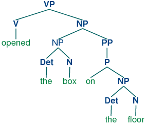
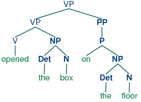
Dynamic programming allows us to build the pp on the floor just once. The first time we build it we save it in a table, then we look it up when we need to use it as a subconstituent of either the object np or the higher vp. This table is known as a well-formed substring table (or WFST for short). We will show how to construct the WFST bottom-up so as to systematically record what syntactic constituents have been found.
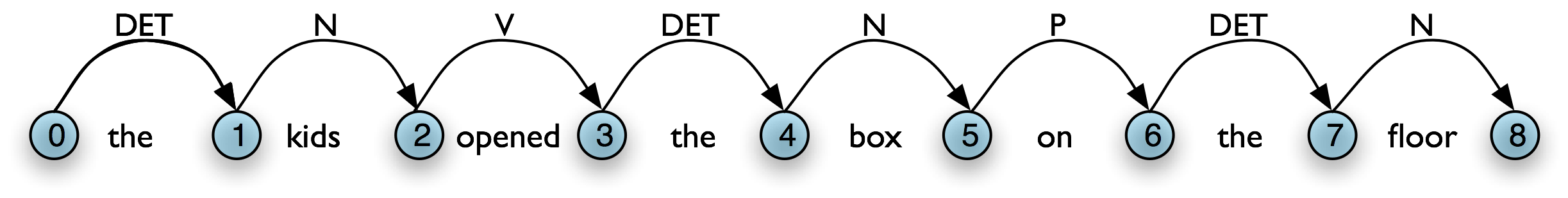
Let's set our input to be the sentence the kids opened the box on the floor. It is helpful to think of the input as being indexed like a Python list. We have illustrated this in Figure 8.2.

Figure 8.2: Slice Points in the Input String
This allows us to say that, for instance, the word opened spans (2, 3) in the input. This is reminiscent of the slice notation:
|
In a WFST, we record the position of the words by filling in cells in a triangular matrix: the vertical axis will denote the start position of a substring, while the horizontal axis will denote the end position (thus opened will appear in the cell with coordinates (2, 3)). To simplify this presentation, we will assume each word has a unique lexical category, and we will store this (not the word) in the matrix. So cell (2, 3) will contain the entry v. More generally, if our input string is a1a2 ... an, and our grammar contains a production of the form A → ai, then we add A to the cell (i-1, i).
So, for every word in tokens, we can look up in our grammar what category it belongs to.
|
For our WFST, we create an (n-1) × (n-1) matrix as a list of lists in Python, and initialize it with the lexical categories of each token, in the init_wfst() function in Listing 8.1. We also define a utility function display() to pretty-print the WFST for us. As expected, there is a v in cell (2, 3).
| ||
| ||
Listing 8.1 (wfst.py): Acceptor Using Well-Formed Substring Table (based on CYK algorithm) |
Returning to our tabular representation, given that we have det in cell (0, 1), and n in cell (1, 2), what should we put into cell (0, 2)? In other words, what syntactic category derives the kids? We have already established that Det derives the and n derives kids, so we need to find a production of the form A → det n, that is, a production whose right hand side matches the categories in the cells we have already found. From the grammar, we know that we can enter np in cell (0,2).
More generally, we can enter A in (i, j) if there is a production A → B C, and we find nonterminal B in (i, k) and C in (k, j). Listing 8.1 uses this inference step to complete the WFST.
Note
To help us easily retrieve productions by their right hand sides, we create an index for the grammar. This is an example of a space-time trade-off: we do a reverse lookup on the grammar, instead of having to check through entire list of productions each time we want to look up via the right hand side.
We conclude that there is a parse for the whole input string once we have constructed an s node that covers the whole input, from position 0 to position 8; i.e., we can conclude that s ⇒* a1a2 ... an.
Notice that we have not used any built-in parsing functions here. We've implemented a complete, primitive chart parser from the ground up!
8.2.2 Charts
By setting trace to True when calling the function complete_wfst(), we get additional output.
|
For example, this says that since we found Det at wfst[0][1] and N at wfst[1][2], we can add NP to wfst[0][2]. The same information can be represented in a directed acyclic graph, as shown in Figure 8.2(a). This graph is usually called a chart. Figure 8.2(b) is the corresponding graph representation, where we add a new edge labeled np to cover the input from 0 to 2.
|
|
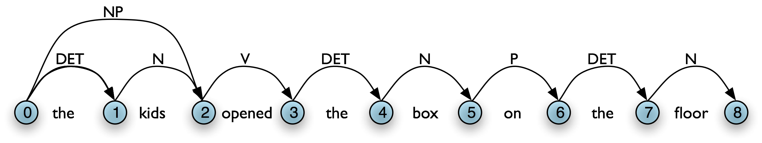
(Charts are more general than the WFSTs we have seen, since they can hold multiple hypotheses for a given span.)
A WFST is a data structure that can be used by a variety of parsing algorithms. The particular method for constructing a WFST that we have just seen and has some shortcomings. First, as you can see, the WFST is not itself a parse tree, so the technique is strictly speaking recognizing that a sentence is admitted by a grammar, rather than parsing it. Second, it requires every non-lexical grammar production to be binary (see Section 8.5.1). Although it is possible to convert an arbitrary CFG into this form, we would prefer to use an approach without such a requirement. Third, as a bottom-up approach it is potentially wasteful, being able to propose constituents in locations that would not be licensed by the grammar. Finally, the WFST did not represent the structural ambiguity in the sentence (i.e. the two verb phrase readings). The vp in cell (2,8) was actually entered twice, once for a v np reading, and once for a vp pp reading. In the next section we will address these issues.
8.2.3 Exercises
- ☼ Consider the sequence of words: Buffalo buffalo Buffalo buffalo buffalo buffalo Buffalo buffalo. This is a grammatically correct sentence, as explained at http://en.wikipedia.org/wiki/Buffalo_buffalo_Buffalo_buffalo_buffalo_buffalo_Buffalo_buffalo. Consider the tree diagram presented on this Wikipedia page, and write down a suitable grammar. Normalize case to lowercase, to simulate the problem that a listener has when hearing this sentence. Can you find other parses for this sentence? How does the number of parse trees grow as the sentence gets longer? (More examples of these sentences can be found at http://en.wikipedia.org/wiki/List_of_homophonous_phrases).
- ◑ Consider the algorithm in Listing 8.1. Can you explain why parsing context-free grammar is proportional to n3?
- ◑ Modify the functions init_wfst() and complete_wfst() so that the contents of each cell in the WFST is a set of non-terminal symbols rather than a single non-terminal.
- ★ Modify the functions init_wfst() and complete_wfst() so that when a non-terminal symbol is added to a cell in the WFST, it includes a record of the cells from which it was derived. Implement a function that will convert a WFST in this form to a parse tree.
8.3 Active Charts
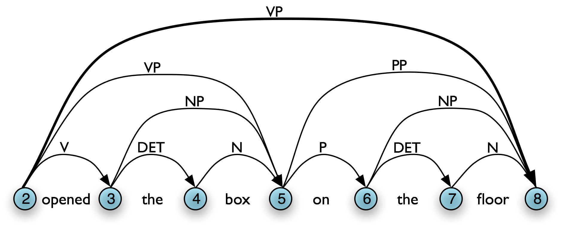
One important aspect of the tabular approach to parsing can be seen more clearly if we look at the graph representation: given our grammar, there are two different ways to derive a top-level vp for the input, as shown in Table 8.3(a,b). In our graph representation, we simply combine the two sets of edges to yield Table 8.3(c).
|
|
|

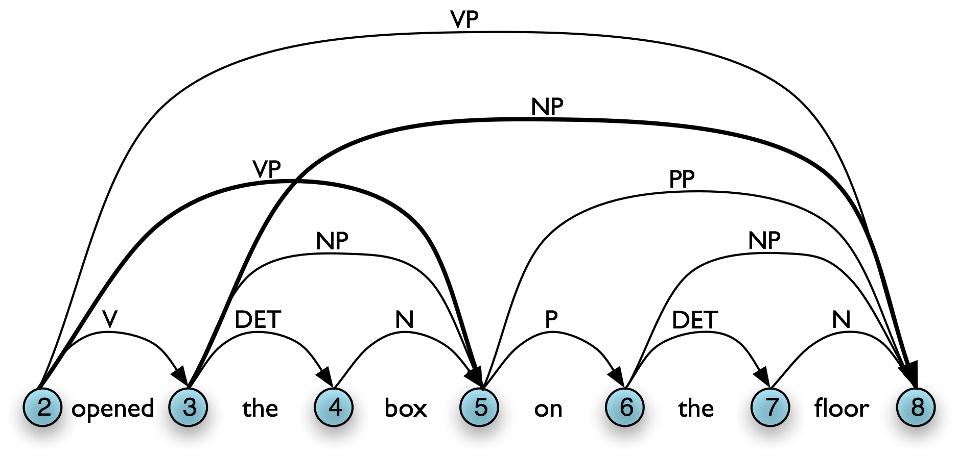
However, given a WFST we cannot necessarily read off the justification for adding a particular edge. For example, in 8.3(b), [Edge: VP, 2:8] might owe its existence to a production vp → v np pp. Unlike phrase structure trees, a WFST does not encode a relation of immediate dominance. In order to make such information available, we can label edges not just with a non-terminal category, but with the whole production that justified the addition of the edge. This is illustrated in Figure 8.3.
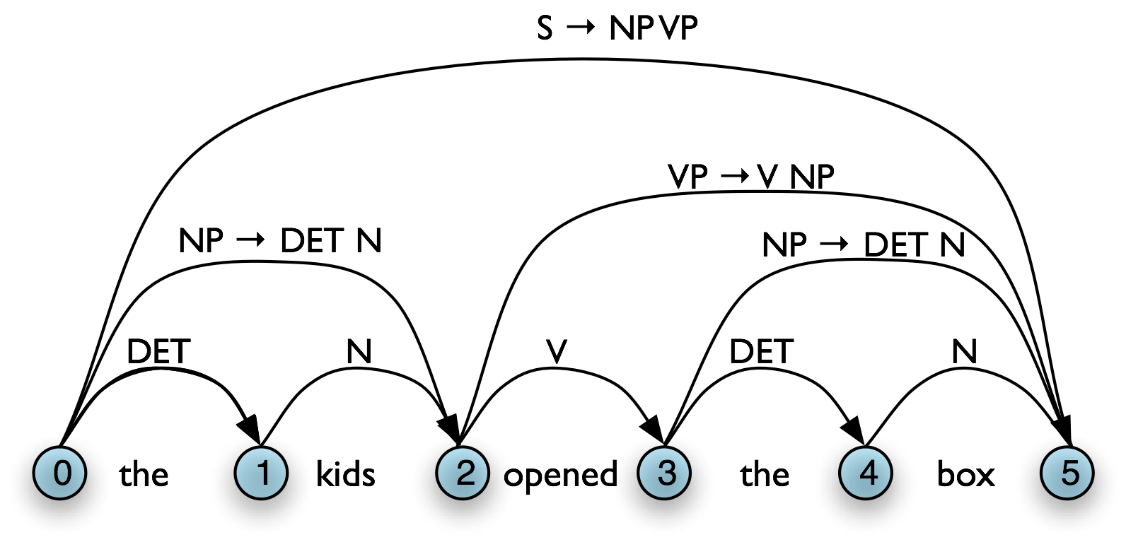
Figure 8.3: Chart Annotated with Productions
In general, a chart parser hypothesizes constituents (i.e. adds edges) based on the grammar, the tokens, and the constituents already found. Any constituent that is compatible with the current knowledge can be hypothesized; even though many of these hypothetical constituents will never be used in the final result. A WFST just records these hypotheses.
All of the edges that we've seen so far represent complete constituents. However, as we will see, it is helpful to hypothesize incomplete constituents. For example, the work done by a parser in processing the production VP → V NP PP can be reused when processing VP → V NP. Thus, we will record the hypothesis that "the v constituent likes is the beginning of a vp."
We can record such hypotheses by adding a dot to the edge's right hand side. Material to the left of the dot specifies what the constituent starts with; and material to the right of the dot specifies what still needs to be found in order to complete the constituent. For example, the edge in the Figure 8.4 records the hypothesis that "a vp starts with the v likes, but still needs an np to become complete":
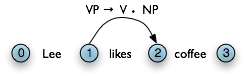
Figure 8.4: Chart Containing Incomplete VP Edge
These dotted edges are used to record all of the hypotheses that a chart parser makes about constituents in a sentence. Formally a dotted edge [A → c1 … cd • cd+1 … cn, (i, j)] records the hypothesis that a constituent of type A with span (i, j) starts with children c1 … cd, but still needs children cd+1 … cn to be complete (c1 … cd and cd+1 … cn may be empty). If d = n, then cd+1 … cn is empty and the edge represents a complete constituent and is called a complete edge. Otherwise, the edge represents an incomplete constituent, and is called an incomplete edge. In Figure 8.4(a), [vp → v np •, (1, 3)] is a complete edge, and [vp → v • np, (1, 2)] is an incomplete edge.
If d = 0, then c1 … cn is empty and the edge is called a self-loop edge. This is illustrated in Table 8.4(b). If a complete edge spans the entire sentence, and has the grammar's start symbol as its left-hand side, then the edge is called a parse edge, and it encodes one or more parse trees for the sentence. In Table 8.4(c), [s → np vp •, (0, 3)] is a parse edge.
a. Incomplete Edge
 |
b. Self Loop Edge
 |
c. Parse Edge
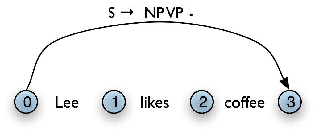 |
8.3.1 The Chart Parser
To parse a sentence, a chart parser first creates an empty chart spanning the sentence. It then finds edges that are licensed by its knowledge about the sentence, and adds them to the chart one at a time until one or more parse edges are found. The edges that it adds can be licensed in one of three ways:
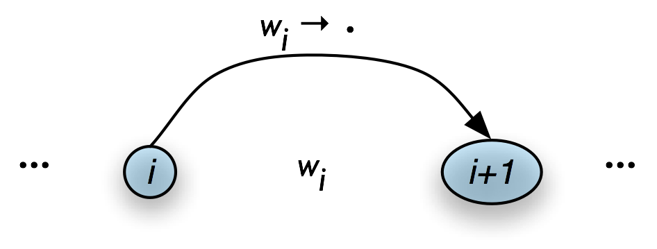
- The input can license an edge. In particular, each word wi in the input licenses the complete edge [wi → •, (i, i+1)].
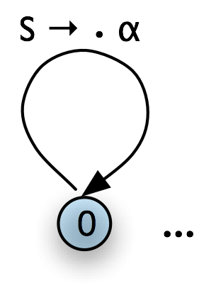
- The grammar can license an edge. In particular, each grammar production A → α licenses the self-loop edge [A → • α, (i, i)] for every i, 0 ≤ i < n.
- The current chart contents can license an edge.
However, it is not wise to add all licensed edges to the chart, since many of them will not be used in any complete parse. For example, even though the edge in the following chart is licensed (by the grammar), it will never be used in a complete parse:
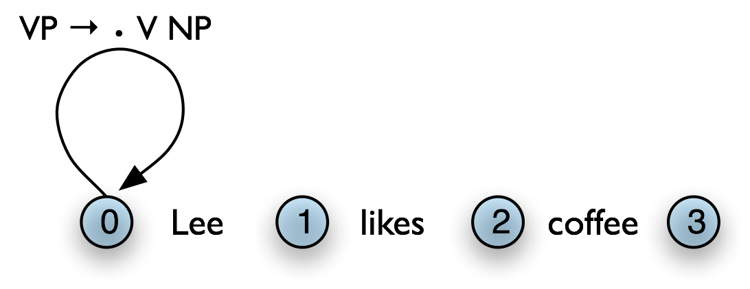
Figure 8.5: Chart Containing Redundant Edge
Chart parsers therefore use a set of rules to heuristically decide when an edge should be added to a chart. This set of rules, along with a specification of when they should be applied, forms a strategy.
8.3.2 The Fundamental Rule
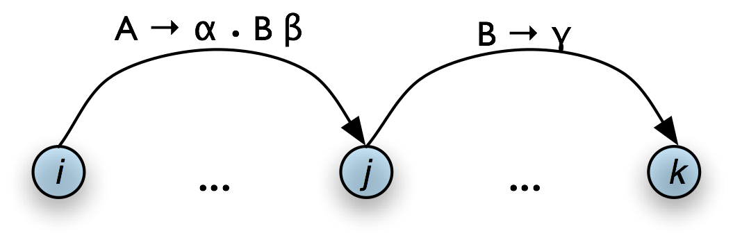
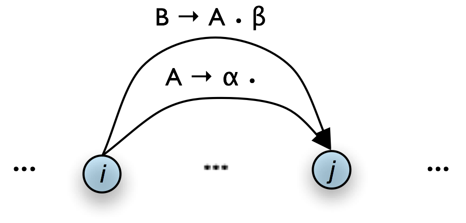
One rule is particularly important, since it is used by every chart parser: the Fundamental Rule. This rule is used to combine an incomplete edge that's expecting a nonterminal B with a following, complete edge whose left hand side is B.
| (3) |
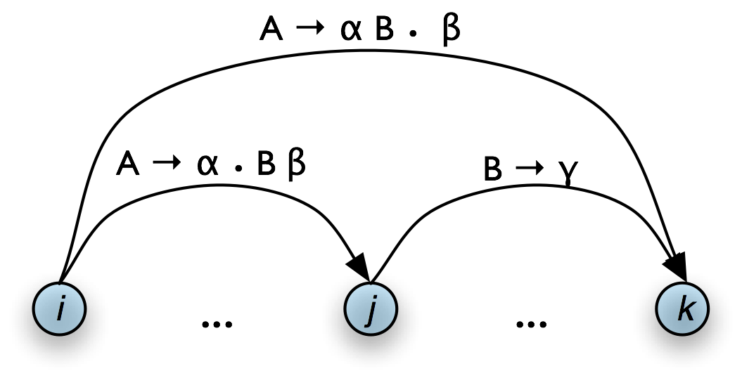
If the chart contains the edges [A → α • B β , (i, j)] [B → γ • , (j, k)] then add the new edge [A → α B • β , (i, k)] where α, β, and γ are (possibly empty) sequences of terminals or non-terminals |
Note that the dot has moved one place to the right, and the span of this new edge is the combined span of the other two. Note also that in adding this new edge we do not remove the other two, because they might be used again.
A somewhat more intuitive version of the operation of the Fundamental Rule can be given using chart diagrams. Thus, if we have a chart of the form shown in Table 8.5(a), then we can add a new complete edge as shown in Table 8.5(b).
a. Input
 |
b. Output
 |
| [1] | The Fundamental Rule corresponds to the Completer function in the Earley algorithm; cf. [Jurafsky & Martin, 2008]. |
8.3.3 Bottom-Up Parsing
As we saw in Chapter 7, bottom-up parsing starts from the input string, and tries to find sequences of words and phrases that correspond to the right hand side of a grammar production. The parser then replaces these with the left-hand side of the production, until the whole sentence is reduced to an S. Bottom-up chart parsing is an extension of this approach in which hypotheses about structure are recorded as edges on a chart. In terms of our earlier terminology, bottom-up chart parsing can be seen as a parsing strategy; in other words, bottom-up is a particular choice of heuristics for adding new edges to a chart.
The general procedure for chart parsing is inductive: we start with a base case, and then show how we can move from a given state of the chart to a new state. Since we are working bottom-up, the base case for our induction will be determined by the words in the input string, so we add new edges for each word. Now, for the induction step, suppose the chart contains an edge labeled with constituent A. Since we are working bottom-up, we want to build constituents that can have an A as a daughter. In other words, we are going to look for productions of the form B → A β and use these to label new edges.
Let's look at the procedure a bit more formally. To create a bottom-up chart parser, we add to the Fundamental Rule two new rules: the Bottom-Up Initialization Rule; and the Bottom-Up Predict Rule. The Bottom-Up Initialization Rule says to add all edges licensed by the input.
| (4) |
For every word wi add the edge [wi → • , (i, i+1)] |
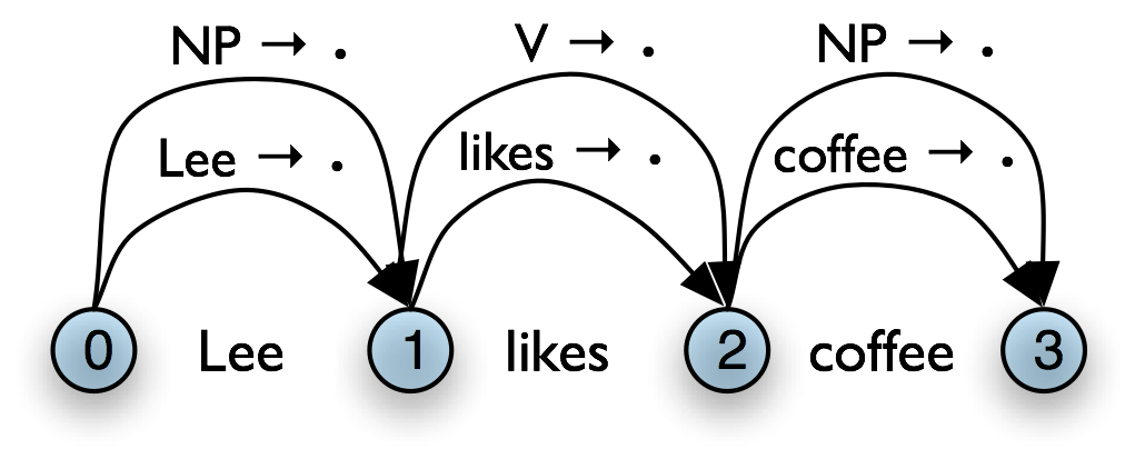
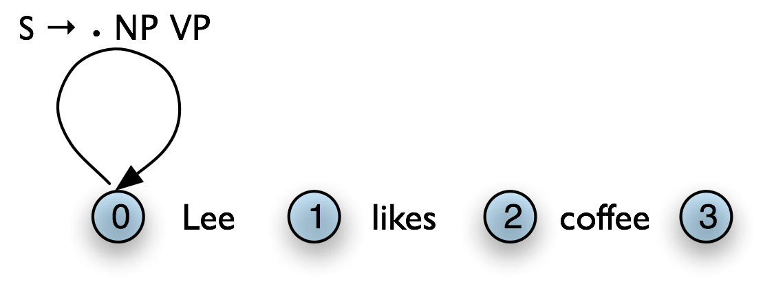
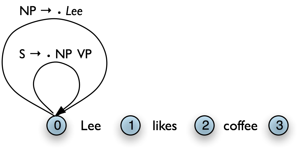
Table 8.6(a) illustrates this rule using the chart notation, while Table 8.6(b) shows the bottom-up initialization for the input Lee likes coffee.
a. Generic
 |
b. Example
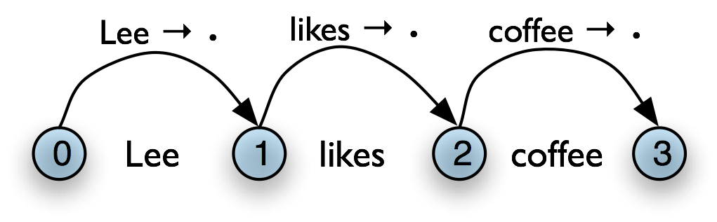 |
Notice that the dot on the right hand side of these productions is telling us that we have complete edges for the lexical items. By including this information, we can give a uniform statement of how the Fundamental Rule operates in Bottom-Up parsing, as we will shortly see.
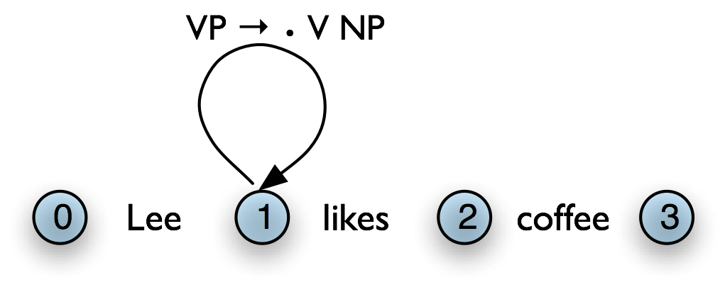
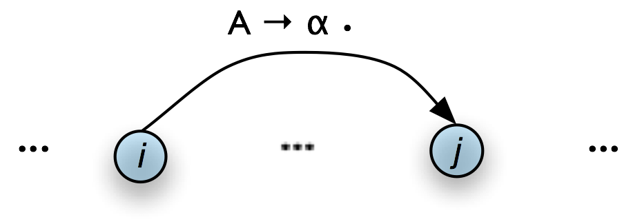
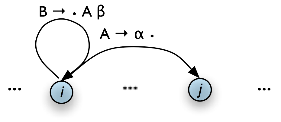
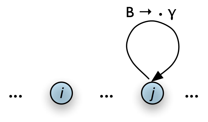
Next, suppose the chart contains a complete edge e whose left hand category is A. Then the Bottom-Up Predict Rule requires the parser to add a self-loop edge at the left boundary of e for each grammar production whose right hand side begins with category A.
| (5) |
If the chart contains the complete edge [A → α • , (i, j)] and the grammar contains the production B → A β then add the self-loop edge [B → • A β , (i, i)] |
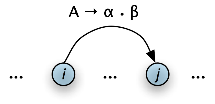
Graphically, if the chart looks as in Figure 8.7(a), then the Bottom-Up Predict Rule tells the parser to augment the chart as shown in Figure 8.7(b).
a. Input
 |
b. Output
 |
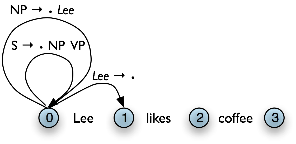
To continue our earlier example, let's suppose that our grammar contains the lexical productions shown in (6a). This allows us to add three self-loop edges to the chart, as shown in (6b).
| (6) |
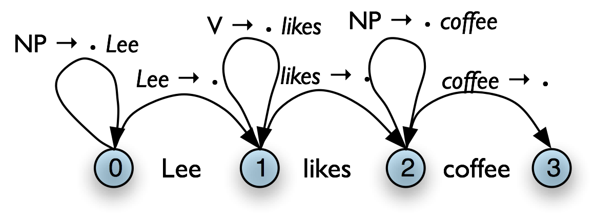 |
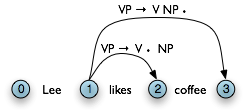
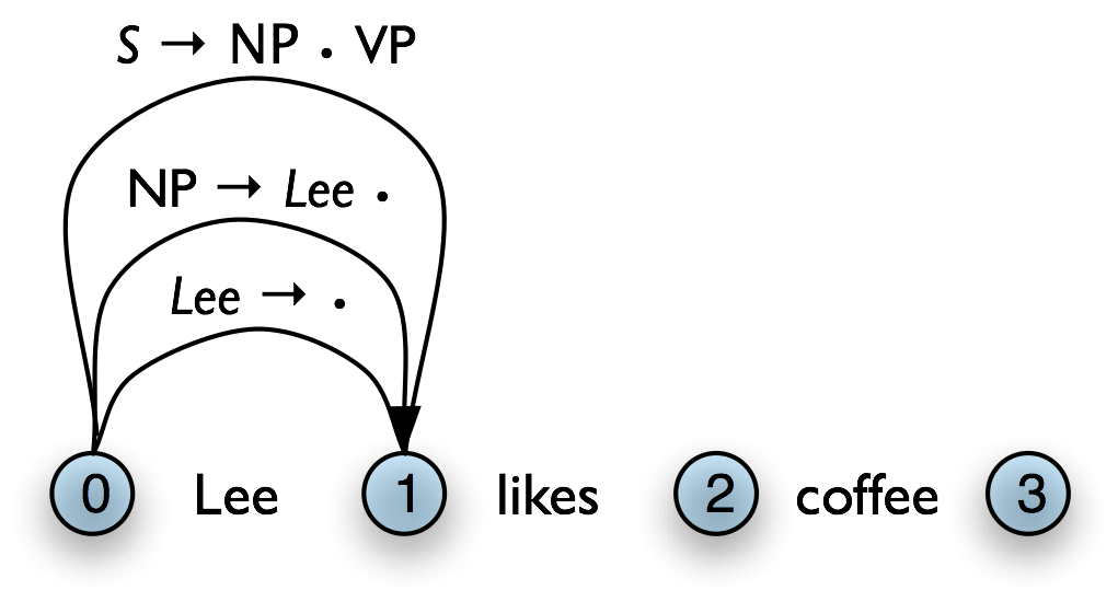
Once our chart contains an instance of the pattern shown in Figure 8.7(b), we can use the Fundamental Rule to add an edge where we have "moved the dot" one position to the right, as shown in Figure 8.8 (we have omitted the self-loop edges for simplicity.)
|
|
We will now be able to add new self-loop edges such as [s → • np vp, (0, 0)] and [vp → • vp np, (1, 1)], and use these to build more complete edges.
Using these three productions, we can parse a sentence as shown in (7).
| (7) |
Create an empty chart spanning the sentence. Apply the Bottom-Up Initialization Rule to each word. Until no more edges are added: Apply the Bottom-Up Predict Rule everywhere it applies. Apply the Fundamental Rule everywhere it applies. Return all of the parse trees corresponding to the parse edges in the chart. |
NLTK provides a useful interactive tool for visualizing the way in which charts are built, nltk.draw.chart.demo(). The tool comes with a pre-defined input string and grammar, but both of these can be readily modified with options inside the Edit menu. Figure 8.6 illustrates a window after the grammar has been updated:
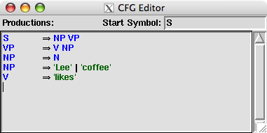
Figure 8.6: Modifying the demo() grammar
Note
To get the symbol ⇒ illustrated in Figure 8.6. you just have to type the keyboard characters '->'.
Figure 8.7 illustrates the tool interface. In order to invoke a rule, you simply click one of the green buttons at the bottom of the window. We show the state of the chart on the input Lee likes coffee after three applications of the Bottom-Up Initialization Rule, followed by successive applications of the Bottom-Up Predict Rule and the Fundamental Rule.
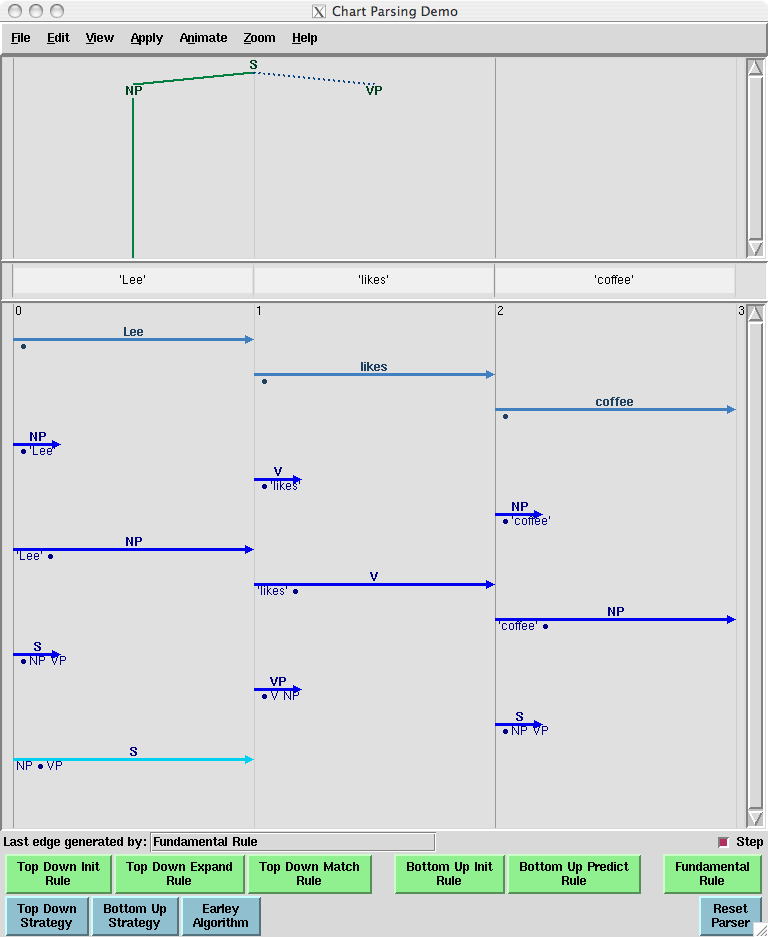
Figure 8.7: Incomplete chart for Lee likes coffee
Notice that in the topmost pane of the window, there is a partial tree showing that we have constructed an s with an np subject in the expectation that we will be able to find a vp.
8.3.4 Top-Down Parsing
Top-down chart parsing works in a similar way to the recursive descent parser discussed in Chapter 7, in that it starts off with the top-level goal of finding an s. This goal is then broken into the subgoals of trying to find constituents such as np and vp that can be immediately dominated by s. To create a top-down chart parser, we use the Fundamental Rule as before plus three other rules: the Top-Down Initialization Rule, the Top-Down Expand Rule, and the Top-Down Match Rule. The Top-Down Initialization Rule in (8) captures the fact that the root of any parse must be the start symbol s. It is illustrated graphically in Table 8.9.
| (8) |
For every grammar production of the form: s → α add the self-loop edge: [s → • α, (0, 0)] |
|
|
As we mentioned before, the dot on the right hand side of a production records how far our goals have been satisfied. So in Figure 8.9(b), we are predicting that we will be able to find an np and a vp, but have not yet satisfied these subgoals. So how do we pursue them? In order to find an np, for instance, we need to invoke a production that has np on its left hand side. The step of adding the required edge to the chart is accomplished with the Top-Down Expand Rule (9). This tells us that if our chart contains an incomplete edge whose dot is followed by a nonterminal B, then the parser should add any self-loop edges licensed by the grammar whose left-hand side is B.
| (9) |
If the chart contains the incomplete edge [A → α • B β , (i, j)] then for each grammar production B → γ add the edge [B → • γ , (j, j)] |
Thus, given a chart that looks like the one in Table 8.10(a), the Top-Down Expand Rule augments it with the edge shown in Table 8.10(b). In terms of our running example, we now have the chart shown in Table 8.10(c).
a. Input
 |
b. Output
 |
c. Example
 |
The Top-Down Match rule allows the predictions of the grammar to be matched against the input string. Thus, if the chart contains an incomplete edge whose dot is followed by a terminal w, then the parser should add an edge if the terminal corresponds to the current input symbol.
| (10) |
If the chart contains the incomplete edge [A → α • wj β, (i, j)], where wj is the j th word of the input, then add a new complete edge [wj → • , (j, j+1)] |
Graphically, the Top-Down Match rule takes us from Table 8.11(a), to Table 8.11(b).
a. Input
 |
b. Output
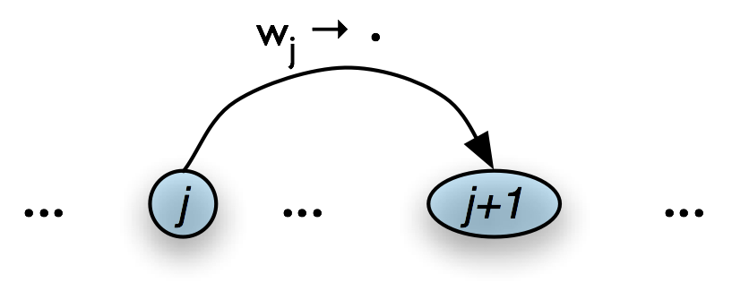 |
Figure 8.12(a) illustrates how our example chart after applying the Top-Down Match rule. What rule is relevant now? The Fundamental Rule. If we remove the self-loop edges from Figure 8.12(a) for simplicity, the Fundamental Rule gives us Figure 8.12(b).
a. Apply Top-Down Match Rule
 |
b. Apply Fundamental Rule
 |
Using these four rules, we can parse a sentence top-down as shown in (11).
| (11) |
Create an empty chart spanning the sentence. Apply the Top-Down Initialization Rule. Until no more edges are added: Apply the Top-Down Expand Rule everywhere it applies. Apply the Top-Down Match Rule everywhere it applies. Apply the Fundamental Rule everywhere it applies. Return all of the parse trees corresponding to the parse edges in the chart. |
We encourage you to experiment with the NLTK chart parser demo, as before, in order to test out the top-down strategy yourself.
8.3.5 The Earley Algorithm
The Earley algorithm [Earley, 1970] is a parsing strategy that resembles the Top-Down Strategy, but deals more efficiently with matching against the input string. Table 8.13 shows the correspondence between the parsing rules introduced above and the rules used by the Earley algorithm.
| Top-Down/Bottom-Up | Earley |
|---|---|
| Top-Down Initialization Rule Top-Down Expand Rule | Predictor Rule |
| Top-Down/Bottom-Up Match Rule | Scanner Rule |
| Fundamental Rule | Completer Rule |
Let's look in more detail at the Scanner Rule. Suppose the chart contains an incomplete edge with a lexical category P immediately after the dot, the next word in the input is w, P is a part-of-speech label for w. Then the Scanner Rule admits a new complete edge in which P dominates w. More precisely:
| (12) |
If the chart contains the incomplete edge [A → α • P β, (i, j)] and wj is the jth word of the input, and P is a valid part of speech for wj, then add the new complete edges [P → wj •, (j, j+1)] [wj → •, (j, j+1)] |
To illustrate, suppose the input is of the form I saw ..., and the chart already contains the edge [vp → • v ..., (1, 1)]. Then the Scanner Rule will add to the chart the edges [v -> 'saw', (1, 2)] and ['saw'→ •, (1, 2)]. So in effect the Scanner Rule packages up a sequence of three rule applications: the Bottom-Up Initialization Rule for [w → •, (j, j+1)], the Top-Down Expand Rule for [P → • wj, (j, j)], and the Fundamental Rule for [P → wj •, (j, j+1))]. This is considerably more efficient than the Top-Down Strategy, that adds a new edge of the form [P → • w , (j, j)] for every lexical rule P → w, regardless of whether w can be found in the input. By contrast with Bottom-Up Initialization, however, the Earley algorithm proceeds strictly left-to-right through the input, applying all applicable rules at that point in the chart, and never backtracking. The NLTK chart parser demo, described above, allows the option of parsing according to the Earley algorithm.
8.3.6 Chart Parsing in NLTK
NLTK defines a simple yet flexible chart parser, ChartParser. A new chart parser is constructed from a grammar and a list of chart rules (also known as a strategy). These rules will be applied, in order, until no new edges are added to the chart. In particular, ChartParser uses the algorithm shown in (13).
| (13) |
Until no new edges are added:
  For each chart rule R:
    Apply R to any applicable edges in the chart.
    Return any complete parses in the chart.
|
nltk.parse.chart defines two ready-made strategies: TD_STRATEGY, a basic top-down strategy; and BU_STRATEGY, a basic bottom-up strategy. When constructing a chart parser, you can use either of these strategies, or create your own.
The following example illustrates the use of the chart parser. We start by defining a simple grammar, and tokenizing a sentence. We make sure it is a list (not an iterator), since we wish to use the same tokenized sentence several times.
| ||
| ||
Listing 8.2 (chart_demo.py): Chart Parsing with NLTK |
The trace parameter can be specified when creating a parser, to turn on tracing (higher trace levels produce more verbose output). Example 8.3 shows the trace output for parsing a sentence with the bottom-up strategy. Notice that in this output, '[-----]' indicates a complete edge, '>' indicates a self-loop edge, and '[----->' indicates an incomplete edge.
| ||
Listing 8.3 (butrace.py): Trace of Bottom-Up Parser |
8.3.7 Exercises
- ☼ Use the graphical chart-parser interface to experiment with different rule invocation strategies. Come up with your own strategy that you can execute manually using the graphical interface. Describe the steps, and report any efficiency improvements it has (e.g. in terms of the size of the resulting chart). Do these improvements depend on the structure of the grammar? What do you think of the prospects for significant performance boosts from cleverer rule invocation strategies?
- ☼ We have seen that a chart parser adds but never removes edges from a chart. Why?
- ◑ Write a program to compare the efficiency of a top-down chart parser compared with a recursive descent parser (Section 7.5.1). Use the same grammar and input sentences for both. Compare their performance using the timeit module (Section 5.5.4).
8.4 Probabilistic Parsing
As we pointed out in the introduction to this chapter, dealing with ambiguity is a key challenge to broad coverage parsers. We have shown how chart parsing can help improve the efficiency of computing multiple parses of the same sentences. But the sheer number of parses can be just overwhelming. We will show how probabilistic parsing helps to manage a large space of parses. However, before we deal with these parsing issues, we must first back up and introduce weighted grammars.
8.4.1 Weighted Grammars
We begin by considering the verb give. This verb requires both a direct object (the thing being given) and an indirect object (the recipient). These complements can be given in either order, as illustrated in example (14b). In the "prepositional dative" form, the indirect object appears last, and inside a prepositional phrase, while in the "double object" form, the indirect object comes first:
| (14) |
|
Using the Penn Treebank sample, we can examine all instances of prepositional dative and double object constructions involving give, as shown in Listing 8.4.
| ||
| ||
Listing 8.4 (give.py): Usage of Give and Gave in the Penn Treebank sample |
We can observe a strong tendency for the shortest complement to appear first. However, this does not account for a form like give NP: federal judges / NP: a raise, where animacy may be playing a role. In fact there turn out to be a large number of contributing factors, as surveyed by [Bresnan & Hay, 2006].
How can such tendencies be expressed in a conventional context free grammar? It turns out that they cannot. However, we can address the problem by adding weights, or probabilities, to the productions of a grammar.
A probabilistic context free grammar (or PCFG) is a context free grammar that associates a probability with each of its productions. It generates the same set of parses for a text that the corresponding context free grammar does, and assigns a probability to each parse. The probability of a parse generated by a PCFG is simply the product of the probabilities of the productions used to generate it.
The simplest way to define a PCFG is to load it from a specially formatted string consisting of a sequence of weighted productions, where weights appear in brackets, as shown in Listing 8.5.
| ||
| ||
Listing 8.5 (pcfg1.py): Defining a Probabilistic Context Free Grammar (PCFG) |
It is sometimes convenient to combine multiple productions into a single line, e.g. VP -> TV NP [0.4] | IV [0.3] | DatV NP NP [0.3]. In order to ensure that the trees generated by the grammar form a probability distribution, PCFG grammars impose the constraint that all productions with a given left-hand side must have probabilities that sum to one. The grammar in Listing 8.5 obeys this constraint: for S, there is only one production, with a probability of 1.0; for VP, 0.4+0.3+0.3=1.0; and for NP, 0.8+0.2=1.0. The parse tree returned by parse() includes probabilities:
|
The next two sections introduce two probabilistic parsing algorithms for PCFGs. The first is an A* parser that uses Viterbi-style dynamic programming to find the single most likely parse for a given text. Whenever it finds multiple possible parses for a subtree, it discards all but the most likely parse. The second is a bottom-up chart parser that maintains a queue of edges, and adds them to the chart one at a time. The ordering of this queue is based on the probabilities associated with the edges, allowing the parser to expand more likely edges before less likely ones. Different queue orderings are used to implement a variety of different search strategies. These algorithms are implemented in the nltk.parse.viterbi and nltk.parse.pchart modules.
8.4.2 A* Parser
An A* Parser is a bottom-up PCFG parser that uses dynamic programming to find the single most likely parse for a text [Klein & Manning, 2003]. It parses texts by iteratively filling in a most likely constituents table. This table records the most likely tree for each span and node value. For example, after parsing the sentence "I saw the man with the telescope" with the grammar cfg.toy_pcfg1, the most likely constituents table contains the following entries (amongst others):
| Span | Node | Tree | Prob |
|---|---|---|---|
| [0:1] | NP | (NP I) | 0.15 |
| [6:7] | NP | (NN telescope) | 0.5 |
| [5:7] | NP | (NP the telescope) | 0.2 |
| [4:7] | PP | (PP with (NP the telescope)) | 0.122 |
| [0:4] | S | (S (NP I) (VP saw (NP the man))) | 0.01365 |
| [0:7] | S | (S (NP I) (VP saw (NP (NP the man) (PP with (NP the telescope))))) | 0.0004163250 |
Once the table has been completed, the parser returns the entry for the most likely constituent that spans the entire text, and whose node value is the start symbol. For this example, it would return the entry with a span of [0:6] and a node value of "S".
Note that we only record the most likely constituent for any given span and node value. For example, in the table above, there are actually two possible constituents that cover the span [1:6] and have "VP" node values.
- "saw the man, who has the telescope":
- (VP saw
- (NP (NP John)
- (PP with (NP the telescope))))
- "used the telescope to see the man":
- (VP saw
- (NP John) (PP with (NP the telescope)))
Since the grammar we are using to parse the text indicates that the first of these tree structures has a higher probability, the parser discards the second one.
Filling in the Most Likely Constituents Table: Because the grammar used by ViterbiParse is a PCFG, the probability of each constituent can be calculated from the probabilities of its children. Since a constituent's children can never cover a larger span than the constituent itself, each entry of the most likely constituents table depends only on entries for constituents with shorter spans (or equal spans, in the case of unary and epsilon productions).
ViterbiParse takes advantage of this fact, and fills in the most likely constituent table incrementally. It starts by filling in the entries for all constituents that span a single element of text. After it has filled in all the table entries for constituents that span one element of text, it fills in the entries for constituents that span two elements of text. It continues filling in the entries for constituents spanning larger and larger portions of the text, until the entire table has been filled.
To find the most likely constituent with a given span and node value, ViterbiParse considers all productions that could produce that node value. For each production, it checks the most likely constituents table for sequences of children that collectively cover the span and that have the node values specified by the production's right hand side. If the tree formed by applying the production to the children has a higher probability than the current table entry, then it updates the most likely constituents table with the new tree.
Handling Unary Productions and Epsilon Productions: A minor difficulty is introduced by unary productions and epsilon productions: an entry of the most likely constituents table might depend on another entry with the same span. For example, if the grammar contains the production V → VP, then the table entries for VP depend on the entries for V with the same span. This can be a problem if the constituents are checked in the wrong order. For example, if the parser tries to find the most likely constituent for a VP spanning [1:3] before it finds the most likely constituents for V spanning [1:3], then it can't apply the V → VP production.
To solve this problem, ViterbiParse repeatedly checks each span until it finds no new table entries. Note that cyclic grammar productions (e.g. V → V) will not cause this procedure to enter an infinite loop. Since all production probabilities are less than or equal to 1, any constituent generated by a cycle in the grammar will have a probability that is less than or equal to the original constituent; so ViterbiParse will discard it.
In NLTK, we create Viterbi parsers using ViterbiParse(). Note that since ViterbiParse only finds the single most likely parse, that nbest_parse() will never return more than one parse.
| ||
| ||
The trace method can be used to set the level of tracing output that is generated when parsing a text. Trace output displays the constituents that are considered, and indicates which ones are added to the most likely constituent table. It also indicates the likelihood for each constituent.
|
8.4.3 A Bottom-Up PCFG Chart Parser
The A* parser described in the previous section finds the single most likely parse for a given text. However, when parsers are used in the context of a larger NLP system, it is often necessary to produce several alternative parses. In the context of an overall system, a parse that is assigned low probability by the parser might still have the best overall probability.
For example, a probabilistic parser might decide that the most likely parse for "I saw John with the cookie" is is the structure with the interpretation "I used my cookie to see John"; but that parse would be assigned a low probability by a semantic system. Combining the probability estimates from the parser and the semantic system, the parse with the interpretation "I saw John, who had my cookie" would be given a higher overall probability.
This section describes a probabilistic bottom-up chart parser. It maintains an edge queue, and adds these edges to the chart one at a time. The ordering of this queue is based on the probabilities associated with the edges, and this allows the parser to insert the most probable edges first. Each time an edge is added to the chart, it may become possible to insert new edges, so these are added to the queue. The bottom-up chart parser continues adding the edges in the queue to the chart until enough complete parses have been found, or until the edge queue is empty.
Like an edge in a regular chart, a probabilistic edge consists of a dotted production, a span, and a (partial) parse tree. However, unlike ordinary charts, this time the tree is weighted with a probability. Its probability is the product of the probability of the production that generated it and the probabilities of its children. For example, the probability of the edge [Edge: S → NP • VP, 0:2] is the probability of the PCFG production S → NP VP multiplied by the probability of its np child. (Note that an edge's tree only includes children for elements to the left of the edge's dot. Thus, the edge's probability does not include probabilities for the constituents to the right of the edge's dot.)
8.4.4 Bottom-Up PCFG Strategies
The edge queue is a sorted list of edges that can be added to the chart. It is initialized with a single edge for each token in the text, with the form [Edge: token |rarr| |dot|]. As each edge from the queue is added to the chart, it may become possible to add further edges, according to two rules: (i) the Bottom-Up Initialization Rule can be used to add a self-loop edge whenever an edge whose dot is in position 0 is added to the chart; or (ii) the Fundamental Rule can be used to combine a new edge with edges already present in the chart. These additional edges are queued for addition to the chart.
By changing the sort order used by the queue, we can control the strategy that the parser uses to explore the search space. Since there are a wide variety of reasonable search strategies, BottomUpChartParser() does not define any sort order. Instead, different strategies are implemented in subclasses of BottomUpChartParser().
Lowest Cost First: The simplest way to order the edge queue is to sort edges by the probabilities of their associated trees (nltk.InsideChartParser()). This ordering concentrates the efforts of the parser on those edges that are more likely to be correct analyses of their underlying tokens.
The probability of an edge's tree provides an upper bound on the probability of any parse produced using that edge. The probabilistic "cost" of using an edge to form a parse is one minus its tree's probability. Thus, inserting the edges with the most likely trees first results in a lowest-cost-first search strategy. Lowest-cost-first search is optimal: the first solution it finds is guaranteed to be the best solution.
However, lowest-cost-first search can be rather inefficient. Recall that a tree's probability is the product of the probabilities of all the productions used to generate it. Consequently, smaller trees tend to have higher probabilities than larger ones. Thus, lowest-cost-first search tends to work with edges having small trees before considering edges with larger trees. Yet any complete parse of the text will necessarily have a large tree, and so this strategy will tend to produce complete parses only once most other edges are processed.
Let's consider this problem from another angle. The basic shortcoming with lowest-cost-first search is that it ignores the probability that an edge's tree will be part of a complete parse. The parser will try parses that are locally coherent even if they are unlikely to form part of a complete parse. Unfortunately, it can be quite difficult to calculate the probability that a tree is part of a complete parse. However, we can use a variety of techniques to approximate that probability.
Best-First Search: This method sorts the edge queue in descending order of the edges' span, no the assumption that edges having a larger span are more likely to form part of a complete parse. Thus, LongestParse employs a best-first search strategy, where it inserts the edges that are closest to producing complete parses before trying any other edges. Best-first search is not an optimal search strategy: the first solution it finds is not guaranteed to be the best solution. However, it will usually find a complete parse much more quickly than lowest-cost-first search.
Beam Search: When large grammars are used to parse a text, the edge queue can grow quite long. The edges at the end of a large well-sorted queue are unlikely to be used. Therefore, it is reasonable to remove (or prune) these edges from the queue. This strategy is known as beam search; it only keeps the best partial results. The bottom-up chart parsers take an optional parameter beam_size; whenever the edge queue grows longer than this, it is pruned. This parameter is best used in conjunction with InsideChartParser(). Beam search reduces the space requirements for lowest-cost-first search, by discarding edges that are not likely to be used. But beam search also loses many of lowest-cost-first search's more useful properties. Beam search is not optimal: it is not guaranteed to find the best parse first. In fact, since it might prune a necessary edge, beam search is not even complete: it is not guaranteed to return a parse if one exists.
In NLTK we can construct these parsers using InsideChartParser, LongestChartParser, RandomChartParser.
| ||
| ||
The trace method can be used to set the level of tracing output that is generated when parsing a text. Trace output displays edges as they are added to the chart, and shows the probability for each edges' tree.
|
8.5 Grammar Induction
As we have seen, PCFG productions are just like CFG productions, adorned with probabilities. So far, we have simply specified these probabilities in the grammar. However, it is more usual to estimate these probabilities from training data, namely a collection of parse trees or treebank.
The simplest method uses Maximum Likelihood Estimation, so called because probabilities are chosen in order to maximize the likelihood of the training data. The probability of a production VP → V NP PP is p(V,NP,PP | VP). We calculate this as follows:
                  count(VP -> V NP PP)
P(V,NP,PP | VP) = --------------------
                  count(VP -> ...)
Here is a simple program that induces a grammar from the first three parse trees in the Penn Treebank corpus:
|
8.5.1 Normal Forms
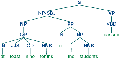
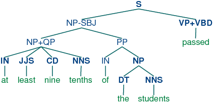
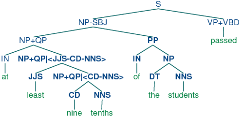
Grammar induction usually involves normalizing the grammar in various ways. NLTK trees support binarization (Chomsky Normal Form), parent annotation, Markov order-N smoothing, and unary collapsing:
|
These trees are shown in (15c).
| (15) |
|
8.6 Conclusion
8.7 Further Reading
Section 13.4 of [Jurafsky & Martin, 2008] covers chart parsing, and Chapter 14 contains a more formal presentation of statistical parsing.
About this document...
This chapter is a draft from Natural Language Processing [http://nltk.org/book.html], by Steven Bird, Ewan Klein and Edward Loper, Copyright © 2008 the authors. It is distributed with the Natural Language Toolkit [http://nltk.org/], Version 0.9.5, under the terms of the Creative Commons Attribution-Noncommercial-No Derivative Works 3.0 United States License [http://creativecommons.org/licenses/by-nc-nd/3.0/us/].
This document is