10.1 Introduction
Imagine you are building a spoken dialogue
system to answer queries about train schedules in Europe. (1)
illustrates one of the input
sentences that the system should handle.
| (1) | | Which stations does the 9.00 express from Amsterdam to Paris stop at? |
The information that the customer is seeking is not exotic — the
system back-end just needs to look up the list of stations on the
route, and reel them off. But you have to be careful in giving the
correct semantic interpretation to
(1). You don't want to end up with the
system trying to answer (2) instead:
| (2) | | Which station does the 9.00 express from Amsterdam terminate at? |
Part of your solution might use domain knowledge to figure out that if
a speaker knows that the train is a train to Paris, then she probably
isn't asking about the terminating station in (1). But the
solution will also involve recognizing the syntactic structure of the
speaker's query. In particular, your analyzer must recognize that
there is a syntactic connection between the question phrase which
stations, and the phrase stop at at the end (1). The
required interpretation is made clearer in the "quiz question version
shown in (3), where the question phrase fills the "gap" that is
implicit in (1):
| (3) | | The 9.00 express from Amsterdam to Paris stops at which stations? |
The long-distance dependency between an initial question phrase
and the gap that it semantically connects to cannot be recognized by
techniques we have presented in earlier chapters. For example, we
can't use n-gram based language models; in practical terms, it is
infeasible to observe the n-grams for a big enough value of
n. Similarly, chunking grammars only attempt to capture local
patterns, and therefore just don't "see" long-distance dependencies.
In this chapter, we will show how syntactic features can be used to
provide a simple yet effective technique for keeping track of
long-distance dependencies in sentences.
Features are helpful too for dealing with purely local dependencies.
Consider the German questions (4).
The only way of telling which noun phrase is the subject of
kennen ('know') and which is the object is by looking at the
agreement inflection on the verb — word order is no help to us
here. Since verbs in German agree in number with their subjects, the
plural form kennen requires Welche Studenten as subject,
while the singular form kennt requires Franz as
subject. The fact that subjects and verbs must agree in number can be
expressed within the CFGs that we presented in Chapter 7. But capturing the fact that the interpretations of
germanagra and germanagrb differ is more challenging. In this
chapter, we will only examine the syntactic aspect of local
dependencies such as number agreement. In Chapter 11, we
will demonstrate how feature-based grammars can be extended so that
they build a representation of meaning in parallel with a
representation of syntactic structure.
Note
Remember that our program samples assume you
begin your interactive session or your program with: import nltk, re, pprint
10.2 Why Features?
We have already used the term "feature" a few times, without saying
what it means. What's special about feature-based grammars? The core
ideas are probably already familiar to you. To make things concrete,
let's look at the simple phrase these dogs. It's composed of two
words. We'll be a bit abstract for the moment, and call these words
a and b. We'll be modest, and assume that we do not know
everything about them, but we can at least give a partial
description. For example, we know that the orthography of a is
these, its phonological form is DH IY Z, its part-of-speech is
Det, and its number is plural. We can use dot notation to record
these observations:
| (5) | |
a.spelling = these
a.phonology = DH IY Z
a.pos = Det
a.number = plural
|
Thus (5) is a partial description of a word; it lists some
attributes, or features, of the word, and declares their values. There
are other attributes that we might be interested in, which have
not been specified; for example, what head the word is dependent on
(using the notion of dependency discussed in Chapter 7), and
what the lemma of the word is. But this omission of some attributes is
exactly what you would expect from a partial description!
We will start off this chapter by looking more closely at the
phenomenon of syntactic agreement; we will show how agreement
constraints can be expressed elegantly using features, and illustrate
their use in a simple grammar. Feature structures are a general data
structure for representing information of any kind; we will briefly
look at them from a more formal point of view, and explain how to
create feature structures in Python. In the final part of the chapter,
we demonstrate that the additional expressiveness of features opens
out a wide spectrum of possibilities for describing sophisticated
aspects of linguistic structure.
10.2.1 Syntactic Agreement
Consider the following contrasts:
In English, nouns are usually morphologically marked as being singular
or plural. The form of the demonstrative also varies:
this (singular) and these (plural).
Examples (6b) and (7b) show that there are constraints on
the use of demonstratives and nouns within a noun phrase:
either both are singular or both are plural. A similar
constraint holds between subjects and predicates:
Here we can see that morphological properties of the verb co-vary
with syntactic properties of the subject noun phrase. This co-variance is
called agreement.
If we look further at verb agreement in English, we will see that
present tense verbs typically have two inflected forms: one for third person
singular, and another for every other combination of person and number:
| |
singular |
plural |
| 1st per |
I run |
we run |
| 2nd per |
you run |
you run |
| 3rd per |
he/she/it
runs |
they run |
Table 10.1:
Agreement Paradigm for English Regular Verbs
We can make the role of morphological properties a bit more explicit
as illustrated in runs and run. These representations indicate that
the verb agrees with its subject in person and number. (We use "3" as
an abbreviation for 3rd person, "SG" for singular and "PL" for plural.)
Let's see what happens when we encode these agreement constraints in a
context-free grammar. We will begin with the simple CFG in (10).
| (10) | |
s → np vp
np → Det n
vp → v

Det → 'this'
n → 'dog'
v → 'runs'
|
Example (10) allows us to generate the sentence this dog runs;
however, what we really want to do is also generate these dogs
run while blocking unwanted strings such as *this dogs run
and *these dog runs. The most straightforward approach is to
add new non-terminals and productions to the grammar:
| (11) | |
S_SG → NP_SG VP_SG
S_PL → NP_PL VP_PL
NP_SG → Det_SG N_SG
NP_PL → Det_PL N_PL
VP_SG → V_SG
VP_PL → V_PL

Det_SG → 'this'
Det_PL → 'these'
N_SG → 'dog'
N_PL → 'dogs'
V_SG → 'runs'
V_PL → 'run'
|
It should be clear that this grammar will do the required
task, but only at the cost of duplicating our previous set of
productions.
10.2.2 Using Attributes and Constraints
We spoke informally of linguistic categories having properties; for
example, that a noun has the property of being plural. Let's
make this explicit:
In (12), we have introduced some new notation which says that the
category N has a feature called num (short for
'number') and that the value of this feature is pl (short for
'plural'). We can add similar annotations to other categories, and use
them in lexical entries:
| (13) | |
Det[num=sg] → 'this'
Det[num=pl]  → 'these'
N[num=sg] → 'dog'
N[num=pl] → 'dogs'
V[num=sg] → 'runs'
V[num=pl] → 'run'
|
Does this help at all? So far, it looks just like a slightly more
verbose alternative to what was specified in (11). Things become
more interesting when we allow variables over feature values, and use
these to state constraints:
| (14) | |
| a. | |
S → NP[num=?n] VP[num=?n]
|
| b. | |
NP[num=?n] → Det[num=?n] N[num=?n]
|
| c. | |
VP[num=?n] → V[num=?n]
|
|
We are using "?n" as a variable over values of num; it can
be instantiated either to sg or pl. Its scope is
limited to individual productions. That is, within (14a), for example,
?n must be instantiated to the same constant value; we can
read the production as saying that whatever value NP takes for the feature
num, VP must take the same value.
In order to understand how these feature constraints work, it's
helpful to think about how one would go about building a tree. Lexical
productions will admit the following local trees (trees of
depth one):
| (15) | |
| a. | |  |
| b. | |  |
|
| (16) | |
| a. | |  |
| b. | |  |
|
Now (14b) says that whatever the num values of N and
Det are, they have to be the same. Consequently, (14b) will
permit (15a) and (16a) to be combined into an NP as shown in
(17a) and it will also allow (15b) and (16b) to be combined, as in
(17b). By contrast, (18a) and (18b) are prohibited because the roots
of their
constituent local trees differ in their values for the num feature.
| (17) | |
| a. | |  |
| b. | |  |
|
| (18) | |
| a. | |  |
| b. | |  |
|
Production (14c) can be thought of as saying that the num value of the
head verb has to be the same as the num value of the VP
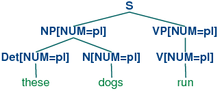
mother. Combined with (14a), we derive the consequence that if the
num value of the subject head noun is pl, then so is
the num value of the VP's head verb.
| (19) | |  |
The grammar in listing 10.1 illustrates most of the ideas we have introduced so
far in this chapter, plus a couple of new ones.
| |
>>> nltk.data.show_cfg('grammars/feat0.fcfg')
% start S
# ############################
# Grammar Rules
# ############################
# S expansion rules
S -> NP[NUM=?n] VP[NUM=?n]
# NP expansion rules
NP[NUM=?n] -> N[NUM=?n]
NP[NUM=?n] -> PropN[NUM=?n]
NP[NUM=?n] -> Det[NUM=?n] N[NUM=?n]
NP[NUM=pl] -> N[NUM=pl]
# VP expansion rules
VP[TENSE=?t, NUM=?n] -> IV[TENSE=?t, NUM=?n]
VP[TENSE=?t, NUM=?n] -> TV[TENSE=?t, NUM=?n] NP
# ############################
# Lexical Rules
# ############################
Det[NUM=sg] -> 'this' | 'every'
Det[NUM=pl] -> 'these' | 'all'
Det -> 'the' | 'some'
PropN[NUM=sg]-> 'Kim' | 'Jody'
N[NUM=sg] -> 'dog' | 'girl' | 'car' | 'child'
N[NUM=pl] -> 'dogs' | 'girls' | 'cars' | 'children'
IV[TENSE=pres,  NUM=sg] -> 'disappears' | 'walks'
TV[TENSE=pres, NUM=sg] -> 'sees' | 'likes'
IV[TENSE=pres,  NUM=pl] -> 'disappear' | 'walk'
TV[TENSE=pres, NUM=pl] -> 'see' | 'like'
IV[TENSE=past, NUM=?n] -> 'disappeared' | 'walked'
TV[TENSE=past, NUM=?n] -> 'saw' | 'liked'
|
|
Listing 10.1 (feat0cfg.py): Example Feature-Based Grammar |
Notice that a syntactic category can have more than one feature; for example,
v[tense=pres, num=pl].
In general, we can add as many features as we like.
Notice also that we have used feature variables in lexical entries as well
as grammatical productions. For example, the has been assigned the
category Det[num=?n]. Why is this? Well,
you know that the definite article the can combine with both
singular and plural nouns. One way of describing this would be to add
two lexical entries to the grammar, one each for the singular and
plural versions of the. However, a more elegant solution is to
leave the num value underspecified and letting it agree
in number with whatever noun it combines with.
A final detail about 10.1 is the statement %start S.
This a "directive" that tells the parser to take s as the
start symbol for the grammar.
In general, when we are trying to develop even a very small grammar,
it is convenient to put the productions in a file where they can be edited,
tested and revised. We have saved 10.1 as a file named
'feat0.fcfg' in the NLTK data distribution, and it
can be accessed using nltk.data.load().
We can inspect the productions and the lexicon using the commands print
g.earley_grammar() and pprint(g.earley_lexicon()).
Next, we can tokenize a sentence and use the nbest_parse() function to
invoke the Earley chart parser.
| |
>>> tokens = 'Kim likes children'.split()
>>> from nltk.parse import load_earley
>>> cp = load_earley('grammars/feat0.fcfg', trace=2)
>>> trees = cp.nbest_parse(tokens)
          |.K.l.c.|
Processing queue 0
Predictor |> . . .| [0:0] S[] -> * NP[NUM=?n] VP[NUM=?n] {}
Predictor |> . . .| [0:0] NP[NUM=?n] -> * N[NUM=?n] {}
Predictor |> . . .| [0:0] NP[NUM=?n] -> * PropN[NUM=?n] {}
Predictor |> . . .| [0:0] NP[NUM=?n] -> * Det[NUM=?n] N[NUM=?n] {}
Predictor |> . . .| [0:0] NP[NUM='pl'] -> * N[NUM='pl'] {}
Scanner   |[-] . .| [0:1] 'Kim'
Scanner   |[-] . .| [0:1] PropN[NUM='sg'] -> 'Kim' *
Processing queue 1
Completer |[-] . .| [0:1] NP[NUM='sg'] -> PropN[NUM='sg'] *
Completer |[-> . .| [0:1] S[] -> NP[NUM=?n] * VP[NUM=?n] {?n: 'sg'}
Predictor |. > . .| [1:1] VP[NUM=?n, TENSE=?t] -> * IV[NUM=?n, TENSE=?t] {}
Predictor |. > . .| [1:1] VP[NUM=?n, TENSE=?t] -> * TV[NUM=?n, TENSE=?t] NP[] {}
Scanner   |. [-] .| [1:2] 'likes'
Scanner   |. [-] .| [1:2] TV[NUM='sg', TENSE='pres'] -> 'likes' *
Processing queue 2
Completer |. [-> .| [1:2] VP[NUM=?n, TENSE=?t] -> TV[NUM=?n, TENSE=?t] * NP[] {?n: 'sg', ?t: 'pres'}
Predictor |. . > .| [2:2] NP[NUM=?n] -> * N[NUM=?n] {}
Predictor |. . > .| [2:2] NP[NUM=?n] -> * PropN[NUM=?n] {}
Predictor |. . > .| [2:2] NP[NUM=?n] -> * Det[NUM=?n] N[NUM=?n] {}
Predictor |. . > .| [2:2] NP[NUM='pl'] -> * N[NUM='pl'] {}
Scanner   |. . [-]| [2:3] 'children'
Scanner   |. . [-]| [2:3] N[NUM='pl'] -> 'children' *
Processing queue 3
Completer |. . [-]| [2:3] NP[NUM='pl'] -> N[NUM='pl'] *
Completer |. [---]| [1:3] VP[NUM='sg', TENSE='pres'] -> TV[NUM='sg', TENSE='pres'] NP[] *
Completer |[=====]| [0:3] S[] -> NP[NUM='sg'] VP[NUM='sg'] *
Completer |[=====]| [0:3] [INIT][] -> S[] *
|
|
Listing 10.2 (featurecharttrace.py): Trace of Feature-Based Chart Parser |
Observe that the parser works directly with
the underspecified productions given by the grammar. That is, the
Predictor rule does not attempt to compile out all admissible feature
combinations before trying to expand the non-terminals on the left hand
side of a production. However, when the Scanner matches an input word
against a lexical production that has been predicted, the new edge will
typically contain fully specified features; e.g., the edge
[PropN[num = sg] → 'Kim', (0, 1)]. Recall from
Chapter 7 that the Fundamental (or Completer) Rule in
standard CFGs is used to combine an incomplete edge that's expecting a
nonterminal B with a following, complete edge whose left hand side
matches B. In our current setting, rather than checking for a
complete match, we test whether the expected category B will
unify with the left hand side B' of a following complete
edge. We will explain in more detail in Section 10.3 how
unification works; for the moment, it is enough to know that as a
result of unification, any variable values of features in B will be
instantiated by constant values in the corresponding feature structure
in B', and these instantiated values will be used in the new edge
added by the Completer. This instantiation can be seen, for example,
in the edge
[np[num=sg] → PropN[num=sg] •, (0, 1)]
in 10.2,
where the feature num has been assigned the value sg.
Finally, we can inspect the resulting parse trees (in this case, a
single one).
| |
>>> for tree in trees: print tree
(S[]
  (NP[NUM='sg'] (PropN[NUM='sg'] Kim))
  (VP[NUM='sg', TENSE='pres']
    (TV[NUM='sg', TENSE='pres'] likes)
    (NP[NUM='pl'] (N[NUM='pl'] children))))
|
|
10.2.3 Terminology
So far, we have only seen feature values like sg and
pl. These simple values are usually called atomic
— that is, they can't be decomposed into subparts. A special
case of atomic values are boolean values, that is, values that
just specify whether a property is true or false of a category. For
example, we might want to distinguish auxiliary verbs such as
can, may, will and do with the boolean feature
aux. Then our lexicon for verbs could include entries such as
(20). (Note that we follow the convention that boolean
features are not written f +, f - but simply
+f, -f, respectively.)
| (20) | |
V[tense=pres, +aux=+] → 'can'
V[tense=pres, +aux=+] → 'may'

V[tense=pres, -aux -] → 'walks'
V[tense=pres, -aux -] → 'likes'
|
We have spoken informally of attaching "feature annotations" to
syntactic categories. A more general
approach is to treat the whole category — that is, the
non-terminal symbol plus the annotation — as a bundle of
features. Consider, for example, the object we have written as (21).
The syntactic category n, as we have seen before, provides part
of speech information. This information can itself be captured as a
feature value pair, using pos to represent "part of speech":
In fact, we regard (22) as our "official" representation of a
feature-based linguistic category, and (21) as a convenient abbreviation.
A bundle of feature-value pairs is called a feature structure
or an attribute value matrix (AVM). A feature structure that
contains a specification for the feature pos is a linguistic
category.
In addition to atomic-valued features, we allow features whose values
are themselves feature structures. For example, we might want to group
together agreement features (e.g., person, number and gender) as a
distinguished part of a category, as shown in (23).
| (23) | |
| |
pos |
= |
N |
|
|
| |
agr |
= |
| |
per |
= |
3 |
|
|
| |
num |
= |
pl |
|
|
| |
gnd |
= |
fem |
|
|
|
|
|
|
In this case, we say that the feature agr has a complex value.
There is no particular significance to the order of features in a
feature structure. So (23) is equivalent to (23).
| (24) | |
| |
agr |
= |
| |
num |
= |
pl |
|
|
| |
per |
= |
3 |
|
|
| |
gnd |
= |
fem |
|
|
|
|
|
| |
pos |
= |
N |
|
|
|
Once we have the possibility of using features like agr, we
can refactor a grammar like 10.1 so that agreement features are
bundled together. A tiny grammar illustrating this point is shown in (25).
| (25) | |
s → np[agr=?n] vp[agr=?n]
np[agr=?n] → PropN[agr=?n]
vp[tense=?t, agr=?n] → Cop[tense=?t, agr=?n] Adj
Cop[tense=pres,  agr=[num=sg, per=3]] → 'is'
PropN[agr=[num=sg, per=3]] → 'Kim'
Adj → 'happy'
|
10.2.4 Exercises
☼ What constraints are required to correctly parse strings like I am
happy and she is happy but not *you is happy or
*they am happy? Implement two solutions for the present tense
paradigm of the verb be in English, first taking Grammar
(11) as your starting point, and then taking Grammar (25)
as the starting point.
☼ Develop a variant of grammar 10.1 that uses a
feature count to make the distinctions shown below:
◑ Develop a feature-based grammar that will correctly describe the following
Spanish noun phrases:
| (30) | |
un
|
cuadro
|
hermos-o
|
INDEF.SG.MASC
|
picture
|
beautiful-SG.MASC
|
'a beautiful picture'
|
|
| (31) | |
un-os
|
cuadro-s
|
hermos-os
|
INDEF-PL.MASC
|
picture-PL
|
beautiful-PL.MASC
|
'beautiful pictures'
|
|
| (32) | |
un-a
|
cortina
|
hermos-a
|
INDEF-SG.FEM
|
curtain
|
beautiful-SG.FEM
|
'a beautiful curtain'
|
|
| (33) | |
un-as
|
cortina-s
|
hermos-as
|
INDEF-PL.FEM
|
curtain
|
beautiful-PL.FEM
|
'beautiful curtains'
|
|
◑ Develop a wrapper for the earley_parser so that a trace
is only printed if the input string fails to parse.
10.3 Computing with Feature Structures
In this section, we will show how feature structures can be
constructed and manipulated in Python. We will also discuss the
fundamental operation of unification, which allows us to combine the
information contained in two different feature structures.
10.3.1 Feature Structures in Python
Feature structures are declared with the
FeatStruct() constructor. Atomic feature values can be strings or
integers.
| |
>>> fs1 = nltk.FeatStruct(TENSE='past', NUM='sg')
>>> print fs1
[ NUM   = 'sg'   ]
[ TENSE = 'past' ]
|
|
A feature structure is actually just a kind of dictionary,
and so we access its values by indexing in the usual way.
We can use our familiar syntax to assign values to features:
| |
>>> fs1 = nltk.FeatStruct(PER=3, NUM='pl', GND='fem')
>>> print fs1['GND']
fem
>>> fs1['CASE'] = 'acc'
|
|
We can also define feature structures that have complex values, as
discussed earlier.
| |
>>> fs2 = nltk.FeatStruct(POS='N', AGR=fs1)
>>> print fs2
[       [ CASE = 'acc' ] ]
[ AGR = [ GND  = 'fem' ] ]
[       [ NUM  = 'pl'  ] ]
[       [ PER  = 3     ] ]
[                        ]
[ POS = 'N'              ]
>>> print fs2['AGR']
[ CASE = 'acc' ]
[ GND  = 'fem' ]
[ NUM  = 'pl'  ]
[ PER  = 3     ]
>>> print fs2['AGR']['PER']
3
|
|
An alternative method of specifying feature structures is to
use a bracketed string consisting of feature-value pairs in the format
feature=value, where values may themselves be feature structures:
| |
>>> nltk.FeatStruct("[POS='N', AGR=[PER=3, NUM='pl', GND='fem']]")
[AGR=[GND='fem', NUM='pl', PER=3], POS='N']
|
|
10.3.2 Feature Structures as Graphs
Feature structures are not inherently tied to linguistic objects; they are
general purpose structures for representing knowledge. For example, we
could encode information about a person in a feature structure:
| |
>>> person01 = nltk.FeatStruct(name='Lee', telno='01 27 86 42 96', age=33)
|
|
| (34) | |
| |
name |
= |
`Lee' |
|
|
| |
telno |
= |
01 27 86 42 96 |
|
|
| |
age |
= |
33 |
|
|
|
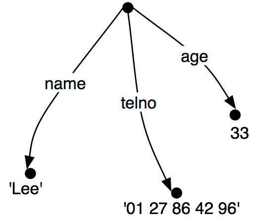
It is sometimes helpful to view feature structures as graphs; more
specifically, directed acyclic graphs (DAGs). (35) is equivalent to
the AVM (34).
| (35) | |  |
The feature names appear as labels on the directed arcs, and feature
values appear as labels on the nodes that are pointed to by the arcs.
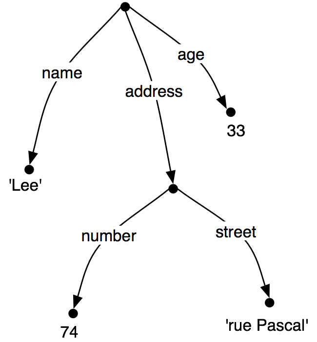
Just as before, feature values can be complex:
| (36) | |  |
When we look at such graphs, it is natural to think in terms of
paths through the graph. A feature path is a sequence of arcs
that can be followed from the root node. We will represent paths as
tuples. Thus, ('address', 'street') is a feature path whose value
in (36) is the string "rue Pascal".
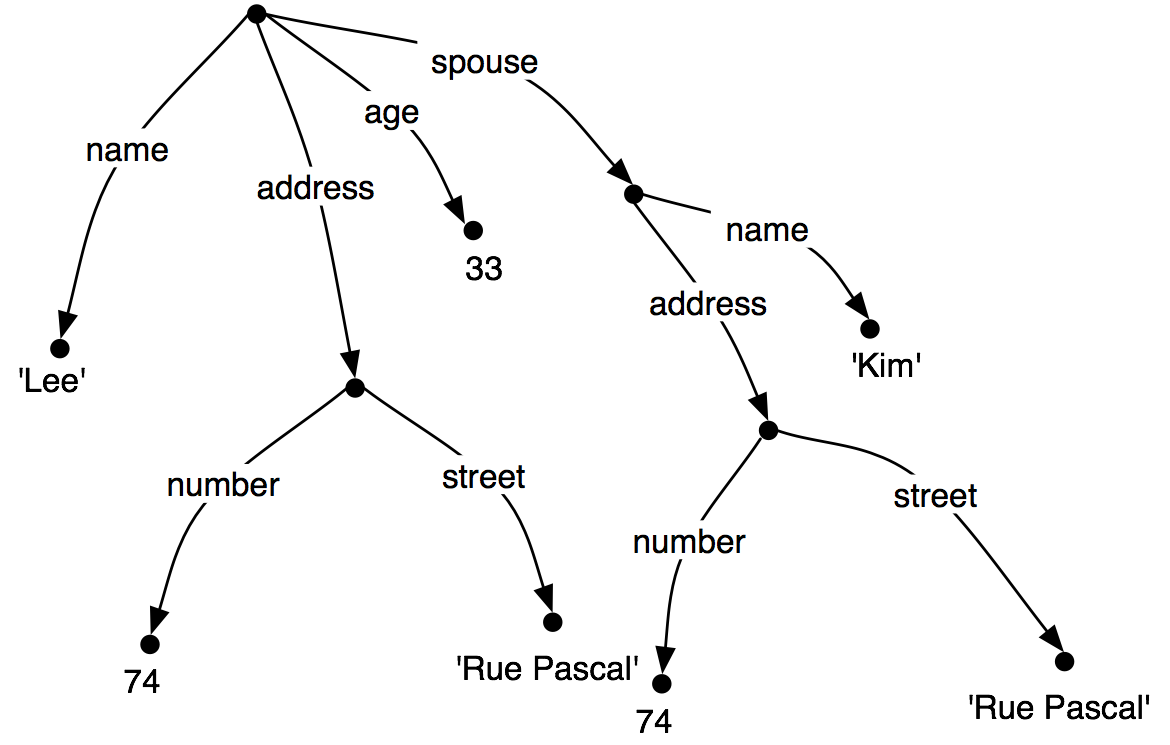
Now let's consider a situation where Lee has a spouse named "Kim", and
Kim's address is the same as Lee's.
We might represent this as (37).
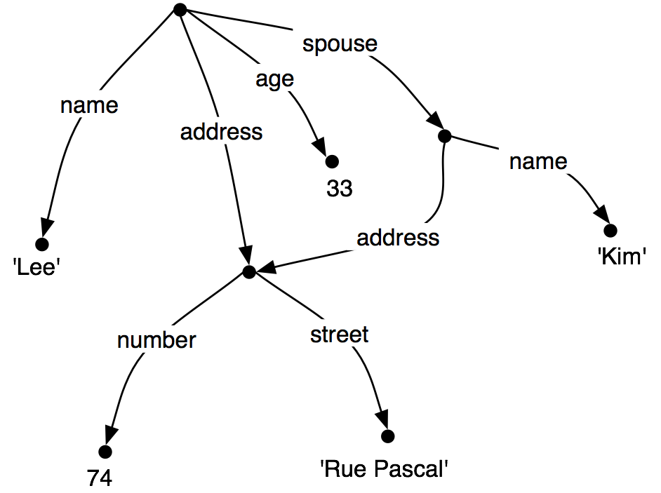
| (37) | |  |
However, rather than repeating the address
information in the feature structure, we can "share" the same
sub-graph between different arcs:
| (38) | |  |
In other words, the value of the path ('ADDRESS') in (38) is
identical to the value of the path ('SPOUSE', 'ADDRESS'). DAGs
such as (38) are said to involve structure sharing or
reentrancy. When two paths have the same value, they are said to
be equivalent.
There are a number of notations for representing reentrancy in
matrix-style representations of feature structures. We adopt
the following convention: the first occurrence of a shared feature structure
is prefixed with an integer in parentheses, such as (1), and any
subsequent reference to that structure uses the notation
->(1), as shown below.
| |
>>> fs = nltk.FeatStruct("""[NAME='Lee', ADDRESS=(1)[NUMBER=74, STREET='rue Pascal'],
...                         SPOUSE=[NAME='Kim', ADDRESS->(1)]]""")
>>> print fs
[ ADDRESS = (1) [ NUMBER = 74           ] ]
[               [ STREET = 'rue Pascal' ] ]
[                                         ]
[ NAME    = 'Lee'                         ]
[                                         ]
[ SPOUSE  = [ ADDRESS -> (1)  ]           ]
[           [ NAME    = 'Kim' ]           ]
|
|
This is similar to more conventional displays of AVMs, as shown in
(39).
| (39) | |
| |
address |
= |
| |
number |
= |
74 |
|
1 |
| |
street |
= |
'rue Pascal' |
|
|
|
|
|
| |
name |
= |
'Lee' |
|
|
| |
spouse |
= |
|
|
|
|
The bracketed integer is sometimes called a tag or a
coindex. The choice of integer is not significant.
There can be any number of tags within a single feature structure.
| |
>>> fs1 = nltk.FeatStruct("[A='a', B=(1)[C='c'], D->(1), E->(1)]")
|
|
10.3.3 Subsumption and Unification
It is standard to think of feature structures as providing partial
information about some object, in the sense that we can order
feature structures according to how general they are. For example,
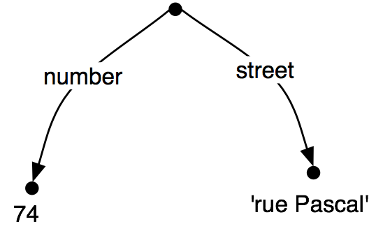
(41a) is more general (less specific) than (41b), which in turn is more general than (41c).
| (41) | |
| b. | |
| |
number |
= |
74 |
|
|
| |
street |
= |
'rue Pascal' |
|
|
|
| c. | |
| |
number |
= |
74 |
|
|
| |
street |
= |
'rue Pascal' |
|
|
| |
city |
= |
'Paris' |
|
|
|
|
This ordering is called subsumption; a more general feature
structure subsumes a less general one. If FS0 subsumes FS1 (formally, we write
FS0 ⊑ FS1), then FS1 must have all the
paths and path equivalences of FS0, and may
have additional paths and equivalences as well. Thus, (37) subsumes
(38), since the latter has additional path equivalences.. It should
be obvious that subsumption only provides a partial ordering on
feature structures, since some feature structures are
incommensurable. For example, (42) neither subsumes nor is subsumed
by (41a).
So we have seen that some feature structures are more specific than
others. How do we go about specializing a given feature structure?
For example, we might decide that addresses should
consist of not just a street number and a street name, but also a
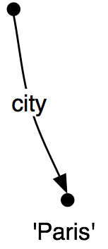
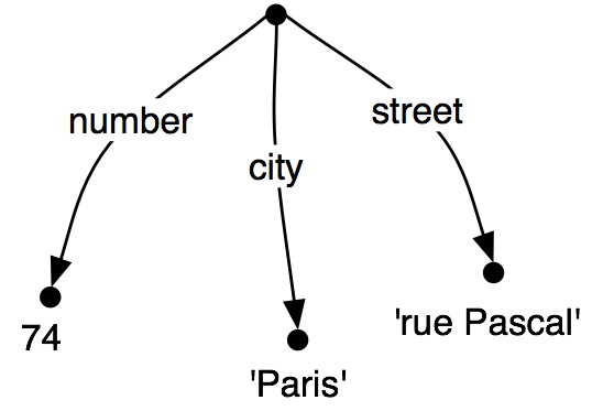
city. That is, we might want to merge graph (43b) with (43a) to
yield (43c).
Merging information from two feature structures is called
unification and is supported by the unify() method.
| |
>>> fs1 = nltk.FeatStruct(NUMBER=74, STREET='rue Pascal')
>>> fs2 = nltk.FeatStruct(CITY='Paris')
>>> print fs1.unify(fs2)
[ CITY   = 'Paris'      ]
[ NUMBER = 74           ]
[ STREET = 'rue Pascal' ]
|
|
Unification is formally defined as a binary operation: FS0 ⊓ FS1. Unification is symmetric, so
| (44) | | FS0 ⊓ FS1 = FS1 ⊓
FS0. |
The same is true in Python:
| |
>>> print fs2.unify(fs1)
[ CITY   = 'Paris'      ]
[ NUMBER = 74           ]
[ STREET = 'rue Pascal' ]
|
|
If we unify two feature structures which stand in the subsumption
relationship, then the result of unification is the most specific of
the two:
| (45) | | If FS0 ⊑ FS1, then FS0
⊓ FS1 = FS1 |
For example, the result of unifying (41b) with (41c) is (41c).
Unification between FS0 and FS1 will fail if the two feature structures share a path π,
but the value of π in FS0 is a distinct
atom from the value of π in FS1.
This is implemented by setting the result of unification to be None.
| |
>>> fs0 = nltk.FeatStruct(A='a')
>>> fs1 = nltk.FeatStruct(A='b')
>>> fs2 = fs0.unify(fs1)
>>> print fs2
None
|
|
Now, if we look at how unification interacts with structure-sharing,
things become really interesting. First, let's define (37) in Python:
| |
>>> fs0 = nltk.FeatStruct("""[NAME=Lee,
...                           ADDRESS=[NUMBER=74,
...                                    STREET='rue Pascal'],
...                           SPOUSE= [NAME=Kim,
...                                    ADDRESS=[NUMBER=74,
...                                             STREET='rue Pascal']]]""")
|
|
| (46) | |
| |
address |
= |
| |
number |
= |
74 |
|
|
| |
street |
= |
`rue Pascal' |
|
|
|
|
|
| |
name |
= |
`Lee' |
|
|
| |
spouse |
= |
| |
address |
= |
| |
number |
= |
74 |
|
|
| |
street |
= |
`rue Pascal' |
|
|
|
|
|
| |
name |
= |
`Kim' |
|
|
|
|
|
|
What happens when we augment Kim's address with a specification
for city? (Notice that fs1 includes the whole path from the root of
the feature structure down to city.)
| |
>>> fs1 = nltk.FeatStruct("[SPOUSE = [ADDRESS = [CITY = Paris]]]")
|
|
(47) shows the result of unifying fs0 with fs1:
| (47) | |
| |
address |
= |
| |
number |
= |
74 |
|
|
| |
street |
= |
`rue Pascal' |
|
|
|
|
|
| |
name |
= |
`Lee' |
|
|
| |
spouse |
= |
| |
address |
= |
| |
city |
= |
`Paris' |
|
|
| |
number |
= |
74 |
|
|
| |
street |
= |
`rue Pascal' |
|
|
|
|
|
| |
name |
= |
`Kim' |
|
|
|
|
|
|
By contrast, the result is very different if fs1 is unified with
the structure-sharing version fs2 (also shown as (38)):
| |
>>> fs2 = nltk.FeatStruct("""[NAME=Lee, ADDRESS=(1)[NUMBER=74, STREET='rue Pascal'],
...                           SPOUSE=[NAME=Kim, ADDRESS->(1)]]""")
|
|
| (48) | |
| |
address |
= |
| |
city |
= |
`Paris' |
|
1 |
| |
number |
= |
74 |
|
|
| |
street |
= |
`rue Pascal' |
|
|
|
|
|
| |
name |
= |
`Lee' |
|
|
| |
spouse |
= |
|
|
|
|
Rather than just updating what was in effect Kim's "copy" of Lee's address,
we have now updated both their addresses at the same time. More
generally, if a unification involves specializing the value of some
path π, then that unification simultaneously specializes the value
of any path that is equivalent to π.
As we have already seen, structure sharing can also be stated
using variables such as ?x.
| |
>>> fs1 = nltk.FeatStruct("[ADDRESS1=[NUMBER=74, STREET='rue Pascal']]")
>>> fs2 = nltk.FeatStruct("[ADDRESS1=?x, ADDRESS2=?x]")
>>> print fs2
[ ADDRESS1 = ?x ]
[ ADDRESS2 = ?x ]
>>> print fs2.unify(fs1)
[ ADDRESS1 = (1) [ NUMBER = 74           ] ]
[                [ STREET = 'rue Pascal' ] ]
[                                          ]
[ ADDRESS2 -> (1)                          ]
|
|
10.3.4 Exercises
☼ Write a function subsumes() which holds of two feature
structures fs1 and fs2 just in case fs1 subsumes fs2.
◑ Consider the feature structures shown in Listing 10.3.
| [XX] | NOTE: This example is somewhat broken -- nltk doesn't support
reentrance for base feature values. (See email ~7/23/08 to the
nltk-users mailing list for details.)
|
| |
fs1 = nltk.FeatStruct("[A = (1)b, B= [C ->(1)]]")
fs2 = nltk.FeatStruct("[B = [D = d]]")
fs3 = nltk.FeatStruct("[B = [C = d]]")
fs4 = nltk.FeatStruct("[A = (1)[B = b], C->(1)]")
fs5 = nltk.FeatStruct("[A = [D = (1)e], C = [E -> (1)] ]")
fs6 = nltk.FeatStruct("[A = [D = (1)e], C = [B -> (1)] ]")
fs7 = nltk.FeatStruct("[A = [D = (1)e, F = (2)[]], C = [B -> (1), E -> (2)] ]")
fs8 = nltk.FeatStruct("[A = [B = b], C = [E = [G = e]]]")
fs9 = nltk.FeatStruct("[A = (1)[B = b], C -> (1)]")
|
|
Listing 10.3 (featstructures.py) |
Work out on paper what the result is of the following
unifications. (Hint: you might find it useful to draw the graph structures.)
- fs1 and fs2
- fs1 and fs3
- fs4 and fs5
- fs5 and fs6
- fs7 and fs8
- fs7 and fs9
Check your answers using Python.
◑ List two feature structures that subsume [A=?x, B=?x].
◑ Ignoring structure sharing, give an informal algorithm for unifying
two feature structures.
10.4 Extending a Feature-Based Grammar
10.4.1 Subcategorization
In Chapter 7, we proposed to augment our
category labels to represent different kinds of verb.
We introduced labels such as iv and tv for intransitive
and transitive verbs respectively. This allowed us to write productions
like the following:
Although we know that iv and tv are two
kinds of v, from a formal point of view
iv has no closer relationship with tv than it does
with np. As it stands, iv and tv are just atomic
nonterminal symbols from a CFG. This approach doesn't allow us
to say anything about the class of verbs in general.
For example, we cannot say something like "All lexical
items of category v can be marked for tense", since bark,
say, is an item of category iv, not v.
A simple solution, originally developed for a grammar framework
called Generalized Phrase Structure Grammar (GPSG), stipulates that lexical
categories may bear a subcat feature whose values are integers.
This is illustrated in a modified portion of 10.1, shown in (50).
| (50) | |
VP[TENSE=?t, NUM=?n] -> V[SUBCAT=0, TENSE=?t, NUM=?n]
VP[TENSE=?t, NUM=?n] -> V[SUBCAT=1, TENSE=?t, NUM=?n] NP
VP[TENSE=?t, NUM=?n] -> V[SUBCAT=2, TENSE=?t, NUM=?n] Sbar

V[SUBCAT=0, TENSE=pres, NUM=sg] -> 'disappears' | 'walks'
V[SUBCAT=1, TENSE=pres, NUM=sg] -> 'sees' | 'likes'
V[SUBCAT=2, TENSE=pres, NUM=sg] -> 'says' | 'claims'

V[SUBCAT=0, TENSE=pres, NUM=pl] -> 'disappear' | 'walk'
V[SUBCAT=1, TENSE=pres, NUM=pl] -> 'see' | 'like'
V[SUBCAT=2, TENSE=pres, NUM=pl] -> 'say' | 'claim'

V[SUBCAT=0, TENSE=past, NUM=?n] -> 'disappeared' | 'walked'
V[SUBCAT=1, TENSE=past, NUM=?n] -> 'saw' | 'liked'
V[SUBCAT=2, TENSE=past, NUM=?n] -> 'said' | 'claimed'
|
When we see a lexical category like v[subcat
1], we can interpret the subcat specification as a
pointer to the production in which v[subcat 1]
is introduced as the head daughter in a vp production.
By convention, there is a one-to-one correspondence between
subcat values and the productions that introduce lexical heads.
It's worth noting that the choice of integer which acts as a value for
subcat is completely arbitrary — we could equally well
have chosen 3999, 113 and 57 as our two values in (50). On this
approach, subcat can only appear on lexical categories; it
makes no sense, for example, to specify a subcat value on
vp.
In our third class of verbs above, we have specified a category
s-bar. This is a label for subordinate clauses such as the
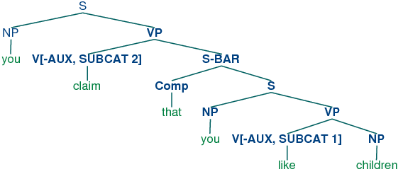
complement of claim in the example You claim that you like
children. We require two further productions to analyze such sentences:
| (51) | |
S-BAR -> Comp S
Comp -> 'that'
|
The resulting structure is the following.
| (52) | |  |
An alternative treatment of subcategorization, due originally to a framework
known as categorial grammar, is represented in feature-based frameworks such as PATR
and Head-driven Phrase Structure Grammar. Rather than using
subcat values as a way of indexing productions, the subcat
value directly encodes the valency of a head (the list of
arguments that it can combine with). For example, a verb like
put that takes np and pp complements (put the
book on the table) might be represented as (53):
| (53) | | v[subcat 〈np, np, pp〉 ] |
This says that the verb can combine with three arguments. The
leftmost element in the list is the subject np, while everything
else — an np followed by a pp in this case — comprises the
subcategorized-for complements. When a verb like put is combined
with appropriate complements, the requirements which are specified in
the subcat are discharged, and only a subject np is
needed. This category, which corresponds to what is traditionally
thought of as vp, might be represented as follows.
Finally, a sentence is a kind of verbal category that has no
requirements for further arguments, and hence has a subcat
whose value is the empty list. The tree (55) shows how these
category assignments combine in a parse of Kim put the book on the table.
| (55) | |  |
10.4.2 Heads Revisited
We noted in the previous section that by factoring subcategorization
information out of the main category label, we could express more
generalizations about properties of verbs. Another property of this
kind is the following: expressions of category v are heads of
phrases of category vp. Similarly (and more informally) ns are heads of nps, as (i.e., adjectives) are heads of aps, and ps (i.e., adjectives) are heads of pps. Not all phrases have
heads — for example, it is standard to say that coordinate
phrases (e.g., the book and the bell) lack heads —
nevertheless, we would like our grammar formalism to express the
mother / head-daughter
relation where it holds. Now, although it looks as though there is
something in common between, say, v and vp, this is more
of a handy convention than a real claim, since v and vp
formally have no more in common than v and Det.
X-bar syntax (cf. [Jacobs & Rosenbaum, 1970], [Jackendoff, 1977]) addresses
this issue by abstracting out the notion of phrasal level. It is
usual to recognize three such levels. If n represents the
lexical level, then n' represents the next level up,
corresponding to the more traditional category Nom, while
n'' represents the phrasal level, corresponding to the
category np. (The primes here replace the typographically more
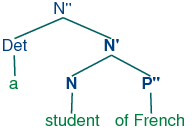
demanding horizontal bars of [Jacobs & Rosenbaum, 1970]). (56) illustrates a
representative structure.
| (56) | |  |
The head of the structure (56) is n while n'
and n'' are called (phrasal) projections of n. n''
is the maximal projection, and n is sometimes called the
zero projection. One of the central claims of X-bar syntax is
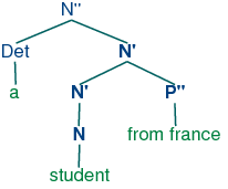
that all constituents share a structural similarity. Using x as
a variable over n, v, a and p, we say that
directly subcategorized complements of the head are always
placed as sisters of the lexical head, whereas adjuncts are
placed as sisters of the intermediate category, x'. Thus, the
configuration of the p'' adjunct in (57) contrasts with that
of the complement p'' in (56).
| (57) | |  |
The productions in (58) illustrate how bar levels can be encoded
using feature structures.
| (58) | |
s → n[bar=2] v[bar=2]
n[bar=2] → Det n[bar=1]
n[bar=1] → n[bar=1] p[bar=2]
n[bar=1] → n[bar=0] p[bar=2]
|
10.4.3 Auxiliary Verbs and Inversion
Inverted clauses — where the order of subject and verb is
switched — occur in English interrogatives and also after
'negative' adverbs:
| (60) | |
| b. | | Never have I seen this dog. |
|
However, we cannot place just any verb in pre-subject position:
Verbs that can be positioned initially in inverted clauses belong to
the class known as auxiliaries, and as well as do,
can and have include be, will and
shall. One way of capturing such structures is with the
following production:
| (63) | |
S[+inv] -> V[+AUX] NP VP
|
That is, a clause marked as [+inv] consists of an auxiliary
verb followed by a vp. (In a more detailed grammar, we would
need to place some constraints on the form of the vp, depending
on the choice of auxiliary.) (64) illustrates the structure of an
inverted clause.
| (64) | |  |
10.4.4 Unbounded Dependency Constructions
Consider the following contrasts:
| (66) | |
| a. | | You put the card into the slot. |
| b. | | *You put into the slot. |
|
The verb like requires an np complement, while
put requires both a following np and pp. Examples
(65) and (66) show that these complements are obligatory:
omitting them leads to ungrammaticality. Yet there are contexts in
which obligatory complements can be omitted, as (67) and (68)
illustrate.
| (67) | |
| a. | | Kim knows who you like. |
| b. | | This music, you really like. |
|
| (68) | |
| a. | | Which card do you put into the slot? |
| b. | | Which slot do you put the card into? |
|
That is, an obligatory complement can be omitted if there is an
appropriate filler in the sentence, such as the question word
who in (67a), the preposed topic this music in (67b), or
the wh phrases which card/slot in (68). It is common to
say that sentences like (67) – (68) contain gaps where
the obligatory complements have been omitted, and these gaps are
sometimes made explicit using an underscore:
| (69) | |
| a. | | Which card do you put __ into the slot? |
| b. | | Which slot do you put the card into __? |
|
So, a gap can occur if it is licensed by a filler. Conversely,
fillers can only occur if there is an appropriate gap elsewhere in
the sentence, as shown by the following examples.
| (70) | |
| a. | | *Kim knows who you like Jody. |
| b. | | *This music, you really like hip-hop. |
|
| (71) | |
| a. | | *Which card do you put this into the slot? |
| b. | | *Which slot do you put the card into this one? |
|
The mutual co-occurence between filler and gap leads to (67) –
(68) is sometimes termed a "dependency". One issue of considerable
importance in theoretical linguistics has been the nature of the
material that can intervene between a filler and the gap that it
licenses; in particular, can we simply list a finite set of strings
that separate the two? The answer is No: there is no upper bound on
the distance between filler and gap. This fact can be easily
illustrated with constructions involving sentential complements, as
shown in (72).
| (72) | |
| b. | | Who do you claim that you like __? |
| c. | | Who do you claim that Jody says that you like __? |
|
Since we can have indefinitely deep recursion of sentential
complements, the gap can be embedded indefinitely far inside the whole
sentence. This constellation of properties leads to the notion of an
unbounded dependency construction; that is, a filler-gap
dependency where there is no upper bound on the distance between
filler and gap.
A variety of mechanisms have been suggested for handling unbounded
dependencies in formal grammars; we shall adopt an approach due to
Generalized Phrase Structure Grammar that involves something called
slash categories. A slash category is something of the form
y/xp; we interpret this as a phrase of category y that
is missing a sub-constituent of category xp. For example,
s/np is an s that is missing an np. The use of
slash categories is illustrated in (73).
| (73) | |  |
The top part of the tree introduces the filler who (treated as
an expression of category np[+wh]) together with a
corresponding gap-containing constituent s/np. The gap information is
then "percolated" down the tree via the vp/np category, until it
reaches the category np/np. At this point, the dependency
is discharged by realizing the gap information as the empty string e
immediately dominated by np/np.
Do we need to think of slash categories as a completely new kind of
object in our grammars? Fortunately, no, we don't — in fact, we
can accommodate them within our existing feature-based framework. We
do this by treating slash as a feature, and the category to its right
as a value. In other words, our "official" notation for s/np
will be s[slash=NP]. Once we have taken this
step, it is straightforward to write a small grammar for
analyzing unbounded dependency constructions. 10.4 illustrates
the main principles of slash categories, and also includes productions for
inverted clauses. To simplify presentation, we have omitted any
specification of tense on the verbs.
| |
>>> nltk.data.show_cfg('grammars/feat1.fcfg')
% start S
# ############################
# Grammar Rules
# ############################
S[-INV] -> NP  S/NP
S[-INV]/?x -> NP VP/?x
S[+INV]/?x -> V[+AUX] NP VP/?x
S-BAR/?x -> Comp S[-INV]/?x
NP/NP ->
VP/?x -> V[SUBCAT=1, -AUX] NP/?x
VP/?x -> V[SUBCAT=2, -AUX] S-BAR/?x
VP/?x -> V[SUBCAT=3, +AUX] VP/?x
# ############################
# Lexical Rules
# ############################
V[SUBCAT=1, -AUX] -> 'see' | 'like'
V[SUBCAT=2, -AUX] -> 'say' | 'claim'
V[SUBCAT=3, +AUX] -> 'do' | 'can'
NP[-WH] -> 'you' | 'children' | 'girls'
NP[+WH] -> 'who'
Comp -> 'that'
|
|
Listing 10.4 (slashcfg.py): Grammar for Simple Long-distance Dependencies |
The grammar in Listing 10.4 contains one gap-introduction production, namely
In order to percolate the slash feature correctly, we need to add
slashes with variable values to both sides of the arrow in productions
that expand s, vp and np. For example,
says that a slash value can be specified on the vp mother of a
constituent if the same value is also specified on the s-bar
daughter. Finally, (76) allows the slash information on np to
be discharged as the empty string.
Using 10.4, we can parse the string who do you claim that you
like into the tree shown in (77).
| (77) | |  |
10.4.5 Case and Gender in German
Compared with English, German has a relatively rich morphology for
agreement. For example, the definite article in German varies with
case, gender and number, as shown in Table 10.2.
| Case |
Masc |
Fem |
Neut |
Plural |
| Nom |
der |
die |
das |
die |
| Gen |
des |
der |
des |
der |
| Dat |
dem |
der |
dem |
den |
| Acc |
den |
die |
das |
die |
Table 10.2:
Morphological Paradigm for the German definite Article
Subjects in German take the nominative case, and most verbs
govern their objects in the accusative case. However, there are
exceptions like helfen that govern the dative case:
| (78) | |
| a. | |
| Die |
Katze |
sieht |
den |
Hund |
| the.NOM.FEM.SG |
cat.3.FEM.SG |
see.3.SG |
the.ACC.MASC.SG |
dog.3.MASC.SG |
| 'the cat sees the dog' |
|
| b. | |
| *Die |
Katze |
sieht |
dem |
Hund |
| the.NOM.FEM.SG |
cat.3.FEM.SG |
see.3.SG |
the.DAT.MASC.SG |
dog.3.MASC.SG |
|
| c. | |
| Die |
Katze |
hilft |
dem |
Hund |
| the.NOM.FEM.SG |
cat.3.FEM.SG |
help.3.SG |
the.DAT.MASC.SG |
dog.3.MASC.SG |
| 'the cat helps the dog' |
|
| d. | |
| *Die |
Katze |
hilft |
den |
Hund |
| the.NOM.FEM.SG |
cat.3.FEM.SG |
help.3.SG |
the.ACC.MASC.SG |
dog.3.MASC.SG |
|
|
The grammar 10.5 illustrates the interaction of agreement
(comprising person, number and gender) with case.
| |
>>> nltk.data.show_cfg('grammars/german.fcfg')
% start S
# Grammar Rules
S -> NP[CASE=nom, AGR=?a] VP[AGR=?a]
NP[CASE=?c, AGR=?a] -> PRO[CASE=?c, AGR=?a]
NP[CASE=?c, AGR=?a] -> Det[CASE=?c, AGR=?a] N[CASE=?c, AGR=?a]
VP[AGR=?a] -> IV[AGR=?a]
VP[AGR=?a] -> TV[OBJCASE=?c, AGR=?a] NP[CASE=?c]
# Lexical Rules
# Singular determiners
# masc
Det[CASE=nom, AGR=[GND=masc,PER=3,NUM=sg]] -> 'der'
Det[CASE=dat, AGR=[GND=masc,PER=3,NUM=sg]] -> 'dem'
Det[CASE=acc, AGR=[GND=masc,PER=3,NUM=sg]] -> 'den'
# fem
Det[CASE=nom, AGR=[GND=fem,PER=3,NUM=sg]] -> 'die'
Det[CASE=dat, AGR=[GND=fem,PER=3,NUM=sg]] -> 'der'
Det[CASE=acc, AGR=[GND=fem,PER=3,NUM=sg]] -> 'die'
# Plural determiners
Det[CASE=nom, AGR=[PER=3,NUM=pl]] -> 'die'
Det[CASE=dat, AGR=[PER=3,NUM=pl]] -> 'den'
Det[CASE=acc, AGR=[PER=3,NUM=pl]] -> 'die'
# Nouns
N[AGR=[GND=masc,PER=3,NUM=sg]] -> 'hund'
N[CASE=nom, AGR=[GND=masc,PER=3,NUM=pl]] -> 'hunde'
N[CASE=dat, AGR=[GND=masc,PER=3,NUM=pl]] -> 'hunden'
N[CASE=acc, AGR=[GND=masc,PER=3,NUM=pl]] -> 'hunde'
N[AGR=[GND=fem,PER=3,NUM=sg]] -> 'katze'
N[AGR=[GND=fem,PER=3,NUM=pl]] -> 'katzen'
# Pronouns
PRO[CASE=nom, AGR=[PER=1,NUM=sg]] -> 'ich'
PRO[CASE=acc, AGR=[PER=1,NUM=sg]] -> 'mich'
PRO[CASE=dat, AGR=[PER=1,NUM=sg]] -> 'mir'
PRO[CASE=nom, AGR=[PER=2,NUM=sg]] -> 'du'
PRO[CASE=nom, AGR=[PER=3,NUM=sg]] -> 'er' | 'sie' | 'es'
PRO[CASE=nom, AGR=[PER=1,NUM=pl]] -> 'wir'
PRO[CASE=acc, AGR=[PER=1,NUM=pl]] -> 'uns'
PRO[CASE=dat, AGR=[PER=1,NUM=pl]] -> 'uns'
PRO[CASE=nom, AGR=[PER=2,NUM=pl]] -> 'ihr'
PRO[CASE=nom, AGR=[PER=3,NUM=pl]] -> 'sie'
# Verbs
IV[AGR=[NUM=sg,PER=1]] -> 'komme'
IV[AGR=[NUM=sg,PER=2]] -> 'kommst'
IV[AGR=[NUM=sg,PER=3]] -> 'kommt'
IV[AGR=[NUM=pl, PER=1]] -> 'kommen'
IV[AGR=[NUM=pl, PER=2]] -> 'kommt'
IV[AGR=[NUM=pl, PER=3]] -> 'kommen'
TV[OBJCASE=acc, AGR=[NUM=sg,PER=1]] -> 'sehe' | 'mag'
TV[OBJCASE=acc, AGR=[NUM=sg,PER=2]] -> 'siehst' | 'magst'
TV[OBJCASE=acc, AGR=[NUM=sg,PER=3]] -> 'sieht' | 'mag'
TV[OBJCASE=dat, AGR=[NUM=sg,PER=1]] -> 'folge' | 'helfe'
TV[OBJCASE=dat, AGR=[NUM=sg,PER=2]] -> 'folgst' | 'hilfst'
TV[OBJCASE=dat, AGR=[NUM=sg,PER=3]] -> 'folgt' | 'hilft'
|
|
Listing 10.5 (germancfg.py): Example Feature-Based Grammar |
- As you will see, the feature objcase is used to
- specify the case that the verb governs on its object.
10.4.6 Exercises
☼ Modify the grammar illustrated in (50) to
incorporate a bar feature for dealing with phrasal projections.
☼ Modify the German grammar in 10.5 to incorporate the
treatment of subcategorization presented in 10.4.1.
◑ Extend the German grammar in 10.5 so that it can
handle so-called verb-second structures like the following:
| (79) | | Heute sieht der hund die katze.
|
★ Morphological paradigms are rarely completely regular, in
the sense of every cell in the matrix having a different
realization. For example, the present tense conjugation of the
lexeme walk only has two distinct forms: walks for the
3rd person singular, and walk for all other combinations of
person and number. A successful analysis should not require
redundantly specifying that 5 out of the 6 possible morphological
combinations have the same realization. Propose and implement a
method for dealing with this.
★ So-called head features are shared between the mother
and head daughter. For example, tense is a head feature
that is shared between a vp and its head v
daughter. See [Gazdar et al, 1985] for more details. Most of the
features we have looked at are head features — exceptions are
subcat and slash. Since the sharing of head
features is predictable, it should not need to be stated explicitly
in the grammar productions. Develop an approach that automatically
accounts for this regular behavior of head features.
10.6 Further Reading
For more examples of feature-based parsing with NLTK, please see the
guides at http://nltk.org/doc/guides/featgram.html,
http://nltk.org/doc/guides/featstruct.html, and
http://nltk.org/doc/guides/grammartestsuites.html.
For an excellent introduction to the phenomenon of agreement, see
[Corbett, 2006].
The earliest use of features in theoretical linguistics was designed
to capture phonological properties of phonemes. For example, a sound
like /b/ might be decomposed into the structure [+labial,
+voice]. An important motivation was to capture
generalizations across classes of segments; for example, that /n/ gets
realized as /m/ preceding any +labial consonant.
Within Chomskyan grammar, it was standard to use atomic features for
phenomena like agreement, and also to capture generalizations across
syntactic categories, by analogy with phonology.
A radical expansion of the use of features in theoretical syntax was
advocated by Generalized Phrase Structure Grammar (GPSG;
[Gazdar et al, 1985]), particularly in the use of features with complex values.
Coming more from the perspective of computational linguistics,
[Dahl & Saint-Dizier, 1985] proposed that functional aspects of language could be
captured by unification of attribute-value structures, and a similar
approach was elaborated by [Grosz & Stickel, 1983] within the PATR-II
formalism. Early work in Lexical-Functional grammar (LFG;
[Bresnan, 1982]) introduced the notion of an f-structure that
was primarily intended to represent the grammatical relations and
predicate-argument structure associated with a constituent structure
parse. [Shieber, 1986] provides an excellent introduction to this
phase of research into feature-based grammars.
One conceptual difficulty with algebraic approaches to feature
structures arose when researchers attempted to model negation. An
alternative perspective, pioneered by [Kasper & Rounds, 1986] and
[Johnson, 1988], argues that grammars involve descriptions of
feature structures rather than the structures themselves. These
descriptions are combined using logical operations such as
conjunction, and negation is just the usual logical operation over
feature descriptions. This description-oriented perspective was
integral to LFG from the outset (cf. [Huang & Chen, 1989], and was also adopted by later
versions of Head-Driven Phrase Structure Grammar (HPSG;
[Sag & Wasow, 1999]). A comprehensive bibliography of HPSG literature can be
found at http://www.cl.uni-bremen.de/HPSG-Bib/.
Feature structures, as presented in this chapter, are unable to
capture important constraints on linguistic information. For example,
there is no way of saying that the only permissible values for
num are sg and pl, while a specification such
as [num=masc] is anomalous. Similarly, we cannot say
that the complex value of agr must contain
specifications for the features per, num and
gnd, but cannot contain a specification such as
[subcat=3]. Typed feature structures were developed to
remedy this deficiency. To begin with, we stipulate that feature
values are always typed. In the case of atomic values, the values just
are types. For example, we would say that the value of num is
the type num. Moreover, num is the most general type of value for
num. Since types are organized hierarchically, we can be more
informative by specifying the value of num is a subtype
of num, namely either sg or pl.
In the case of complex values, we say that feature structures are
themselves typed. So for example the value of agr will be a
feature structure of type agr. We also stipulate that all and only
per, num and gnd are appropriate features for
a structure of type agr. A good early review of work on typed
feature structures is [Emele & Zajac, 1990]. A more comprehensive examination of
the formal foundations can be found in [Carpenter, 1992], while
[Copestake, 2002] focuses on implementing an HPSG-oriented approach
to typed feature structures.
There is a copious literature on the analysis of German within
feature-based grammar frameworks. [Nerbonne, Netter, & Pollard, 1994] is a good
starting point for the HPSG literature on this topic, while
[M{\"u}ller, 2002] gives a very extensive and detailed analysis of
German syntax in HPSG.
Chapter 15 of [Jurafsky & Martin, 2008] discusses feature structures,
the unification algorithm, and the integration of unification into
parsing algorithms.
