11   Logical Semantics

11.1   Introduction

There are many NLP applications where it would be useful to have some representation of the meaning of a natural language sentence. For instance, current search engine technology can only take us so far in giving concise and correct answers to many questions that we might be interested in. Admittedly, Google does a good job in answering (1a), since its first hit is (1b).

By contrast, the result of sending (2) to Google is less helpful:

This time, the topmost hit (and the only relevant one in the top ten) presents the relevant information as a map of the Mediterranean basin. Since the map is an image file, it is not easy to extract the required list of countries from the returned page.

Even if Google succeeds in finding documents which contain information relevant to our question, there is no guarantee that it will be in a form which can be easily converted into an appropriate answer. One reason for this is that the information may have to be inferred from more than one source. This is likely to be the case when we seek an answer to more complex questions like (3):

Here, we would probably need to combine the results of two subqueries, namely (2) and Which countries are in Asia?.

The example queries we have just given are based on a paper dating back to 1982 [Warren & Pereira, 1982]; this describes a system, Chat-80, which converts natural language questions into a semantic representation, and uses the latter to retrieve answers from a knowledge base. A knowledge base is usually taken to be a set of sentences in some formal language; in the case of Chat-80, it is a set of Prolog clauses. However, we can encode knowledge in a variety of formats, including relational databases, various kinds of graph, and first-order models. In NLTK, we have used the third of these options to re-implement a limited version of Chat-80:

Sentence: which Asian countries border the_Mediterranean
------------------------------
\x.((contain(asia, x) & country (x)) & border (x, mediterranean)
set(['turkey', 'syria', 'israel', 'lebanon'])

As we will explain later in this chapter, a semantic representation of the form \x.P(x) denotes a set of entities u that meet some condition P(x). We then ask our knowledge base to enumerate all the entities in this set.

Let's assume more generally that knowledge is available in some structured fashion, and that it can be interrogated by a suitable query language. Then the challenge for NLP is to find a method for converting natural language questions into the target query language. An alternative paradigm for question answering is to take something like the pages returned by a Google query as our 'knowledge base' and then to carry out further analysis and processing of the textual information contained in the returned pages to see whether it does in fact provide an answer to the question. In either case, it is very useful to be able to build a semantic representation of questions. This NLP challenge intersects in interesting ways with one of the key goals of linguistic theory, namely to provide a systematic correspondence between form and meaning.

A widely adopted approach to representing meaning — or at least, some aspects of meaning — involves translating expressions of natural language into first-order logic (FOL). From a computational point of view, a strong argument in favor of FOL is that it strikes a reasonable balance between expressiveness and logical tractability. On the one hand, it is flexible enough to represent many aspects of the logical structure of natural language. On the other hand, automated theorem proving for FOL has been well studied, and although inference in FOL is not decidable, in practice many reasoning problems are efficiently solvable using modern theorem provers (cf. [Blackburn & Bos, 2005] for discussion).

While there are numerous subtle and difficult issues about how to translate natural language constructions into FOL, we will largely ignore these. The main focus of our discussion will be on a different issue, namely building semantic representations which conform to some version of the Principle of Compositionality. (See [Gleitman & Liberman, 1995] for this formulation.)

Principle of Compositionality:

The meaning of a whole is a function of the meanings of the parts and of the way they are syntactically combined.

There is an assumption here that the semantically relevant parts of a complex expression will be determined by a theory of syntax. Within this chapter, we will take it for granted that expressions are parsed against a context-free grammar. However, this is not entailed by the Principle of Compositionality. To summarize, we will be concerned with the task of systematically constructing a semantic representation in a manner that can be smoothly integrated with the process of parsing.

The overall framework we are assuming is illustrated in Figure (4). Given a syntactic analysis of a sentence, we can build one or more semantic representations for the sentence. Once we have a semantic representation, we can also check whether it is true in a model.

(4)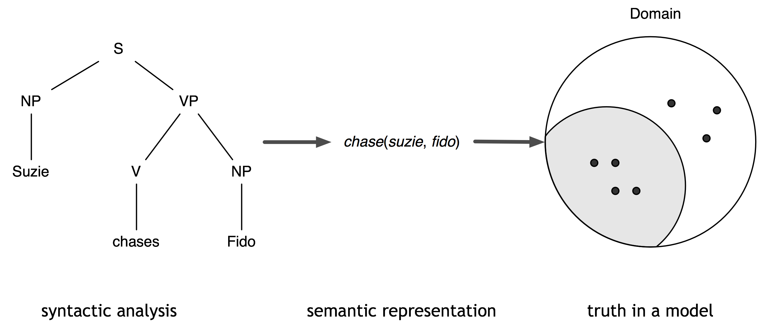

A model for a logical language is a set-theoretic construction which provides a very simplified picture of how the world is. For example, in this case, the model should contain individuals (indicated in the diagram by small dots) corresponding to Suzie and Fido, and it should also specify that these individuals belong to the chase relation.

The order of sections in this chapter is not what you might expect from looking at the diagram. We will start off in the middle of (4) by presenting a logical language that will provide us with semantic representations in NLTK. Next, we will show how formulas in the language can be systematically evaluated in a model. At the end, we will bring everything together and describe a simple method for constructing semantic representations as part of the parse process in NLTK.

11.2   Propositional Logic

The language of propositional logic represents certain aspects of natural language, but at a high level of abstraction. The only structure that is made explicit involves logical connectives; these correspond to 'logically interesting' expressions such as and and not. The basic expressions of the language are propositional variables, usually written p, q, r, etc. Let A be a finite set of such variables. There is a disjoint set of logical connectives which contains the unary operator ¬ (not), and binary operators ∧ (and), ∨ (or), → (implies) and ≡ (iff).

There are many sentences of English which could be taken to have the logical structure shown in (5). Here's an example:

In order to explain the relation between (5) and (6), we need to give a key which maps between propositional variables and English sentences:

The Boolean connectives of propositional logic are supported by the sem package, and are parsed into various kinds of Expression. We use -, &, |, ->, <-> to stand, respectively, for not, and, or, implies and iff. In the following example, we start off by creating a new instance lp of the NLTK LogicParser().

>>> lp = nltk.LogicParser()
>>> lp.parse('-(p & q)')
<NegatedExpression -(p & q)>
>>> lp.parse('p & q')
<AndExpression (p & q)>
>>> lp.parse('p | (r -> q)')
<OrExpression (p | (r -> q))>
>>> lp.parse('p <-> -- p')
<IffExpression (p <-> --p)>

As the name suggests, propositional logic only studies the logical structure of formulas made up of atomic propositions. We saw, for example, that propositional variables stood for whole clauses in English. In order to look at how predicates combine with arguments, we need to look at a more complex language for semantic representation, namely first-order logic. In order to show how this new language interacts with the λ-calculus, it will be useful to introduce the notion of types into our syntactic definition, in departure from the rather simple approach to defining the clauses of L_prop.

In the general case, we interpret sentences of a logical language relative to a model, which is a very simplified version of the world. A model for propositional logic needs to assign the values True or False to every possible formula. We do this inductively: first, every propositional variable is assigned a value, and then we compute the value of complex formulas by consulting the meanings of the Boolean connectives and applying them to the values of the formula's components. Let's create a valuation:

>>> val1 = nltk.sem.Valuation([('p', True), ('q', True), ('r', False)])

We initialize a Valuation with a list of pairs, each of which consists of a semantic symbol and a semantic value. The resulting object is essentially just a dictionary that maps logical expressions (treated as strings) to appropriate values.

>>> val1['p']
True

The keys of the dictionary (sorted alphabetically) can also be accessed via the property symbols:

>>> val1.symbols
['p', 'q', 'r']

As we will see later, our models need to be somewhat more complicated in order to handle the more complicated expressions discussed in the next section, so for the time being, just ignore the dom1 and g1 variables in the following declarations.

>>> dom1 = set([])
>>> g = nltk.sem.Assignment(dom1)

Now, let's create a model m that uses ``val1:

>>> m1 = nltk.sem.Model(dom1, val1, prop=True)

The prop=True is just a flag to say that our models are intended for propositional logic.

Every instance of Model defines appropriate truth functions for the Boolean connectives (and in fact they are implemented as functions named AND(), IMPLIES() and so on).

>>> m1.AND
<bound method Model.AND of (set([]), {'q': True, 'p': True, 'r': False})>

We can use these functions to create truth tables:

>>> for first in [True, False]:
...     for second in [True, False]:
...         print "%s %s => %s" % (first, second, m1.AND(first, second))
True True => True
True False => False
False True => False
False False => False

11.3   First-Order Logic

>>> parsed = lp.parse('see(a, b)')
>>> parsed.argument
<IndividualVariableExpression b>
>>> parsed.function
<ApplicationExpression see(a)>
>>> parsed.function.function
<VariableExpression see>

>>> dom2 = set(['b1', 'g1', 'd1'])

>>> v = [('adam','b1'),('betty','g1'),('fido','d1'),
... ('boy',set(['b1'])),('girl',set(['g1'])), ('dog',set(['d1'])),
... ('walk',set(['g1', 'd1'])),
... ('see', set([('b1','g1'),('d1','b1'),('g1','d1'),]))]
>>> val2 = nltk.sem.Valuation(v)
>>> print val2
{'adam': 'b1',
 'betty': 'g1',
 'boy': set([('b1',)]),
 'dog': set([('d1',)]),
 'fido': 'd1',
 'girl': set([('g1',)]),
 'see': set([('b1', 'g1'), ('d1', 'b1'), ('g1', 'd1')]),
 'walk': set([('d1',), ('g1',)])}

>>> from nltk.sem import app
>>> boy = val2['boy']
>>> app(boy, 'b1')
True
>>> app(boy, 'g1')
False
>>> see = val2['see']
>>> app(see, 'g1')
set([('d1',)])
>>> app(app(see, 'g1'), 'd1')
True

>>> g = nltk.sem.Assignment(dom2, [('x', 'b1'), ('y', 'd1')])
>>> g
{'y': 'd1', 'x': 'b1'}

>>> print g
g[d1/y][b1/x]

>>> m2 = nltk.sem.Model(dom2, val2)
>>> m2.evaluate('see(betty, y)', g)
True

>>> g['y']
'd1'

>>> m2.evaluate('see(x, y)', g)
False

>>> g.purge()
>>> g
{}

>>> m2.evaluate('see(adam, y)', g)
'Undefined'

>>> m2.evaluate('some x.(girl(x) & walk(x))', g)
True

>>> m2.evaluate('girl(x) & walk(x)', g.add('x', 'g1'))
True

>>> fmla1 = lp.parse('girl(x) | boy(x)')
>>> m2.satisfiers(fmla1, 'x', g)
set(['b1', 'g1'])
>>> fmla2 = lp.parse('girl(x) -> walk(x)')
>>> m2.satisfiers(fmla2, 'x', g)
set(['b1', 'g1', 'd1'])
>>> fmla3 = lp.parse('walk(x) -> girl(x)')
>>> m2.satisfiers(fmla3, 'x', g)
set(['b1', 'g1'])

>>> for first in [True, False]:
...     for second in [True, False]:
...         print "%s %s => %s" % (first, second, m2.IMPLIES(first, second))
True True => True
True False => False
False True => True
False False => True

>>> m2.evaluate('all x.(girl(x) -> walk(x))', g)
True

11.3.4   Quantificatier Scope Ambiguity

What happens when we want to give a formal representation of a sentence with two quantifiers, such as the following?

(12)

Every girl chases a dog.

There are (at least) two ways of expressing (12) in FOL:

(13)

a. ∀x.((girl x) → ∃y.((dog y) ∧ (chase y x))) b. ∃y.((dog y) ∧ ∀x.((every x) → (chase y x)))

Can we use both of these? Then answer is Yes, but they have different meanings. (13b) is logically stronger than (13a): it claims that there is a unique dog, say Fido, which is chased by every girl. (13a), on the other hand, just requires that for every girl g, we can find some dog which d chases; but this could be a different dog in each case. We distinguish between (13a) and (13b) in terms of the scope of the quantifiers. In the first, ∀ has wider scope than ∃, while in (13b), the scope ordering is reversed. So now we have two ways of representing the meaning of (12), and they are both quite legitimate. In other words, we are claiming that (12) is ambiguous with respect to quantifier scope, and the formulas in (13) give us a formal means of making the two readings explicit. However, we are not just interested in associating two distinct representations with (12). We also want to show in detail how the two representations lead to different conditions for truth in a formal model.

In order to examine the ambiguity more closely, let's fix our valuation as follows:

>>> v3 = [('john', 'b1'), ... ('mary', 'g1'), ... ('suzie', 'g2'), ... ('fido', 'd1'), ... ('tess', 'd2'), ... ('noosa', 'n'), ... ('girl', set(['g1', 'g2'])), ... ('boy', set(['b1', 'b2'])), ... ('dog', set(['d1', 'd2'])), ... ('bark', set(['d1', 'd2'])), ... ('walk', set(['b1', 'g2', 'd1'])), ... ('chase', set([('b1', 'g1'), ('b2', 'g1'), ('g1', 'd1'), ('g2', 'd2')])), ... ('see', set([('b1', 'g1'), ('b2', 'd2'), ('g1', 'b1'), ... ('d2', 'b1'), ('g2', 'n')])), ... ('in', set([('b1', 'n'), ('b2', 'n'), ('d2', 'n')])), ... ('with', set([('b1', 'g1'), ('g1', 'b1'), ('d1', 'b1'), ('b1', 'd1')]))] >>> val3 = nltk.sem.Valuation(v3)

We can use the graph in (14) to visualize the chase relation.

(14)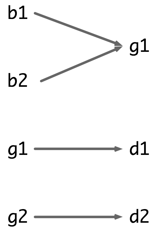

In (14), an arrow between two individuals x and y indicates that x chases y. So b1 and b2 both chase g1, while g1 chases d1 and g2 chases d2. In this model, formula scope2a_ above is true but scope2b_ is false. One way of exploring these results is by using the satisfiers() method of Model objects.

>>> dom3 = val3.domain >>> m3 = nltk.sem.Model(dom3, val3) >>> g = nltk.sem.Assignment(dom3) >>> fmla1 = lp.parse('(girl(x) -> exists y.(dog(y) and chase(x, y)))') >>> m3.satisfiers(fmla1, 'x', g) set(['g2', 'g1', 'n', 'b1', 'b2', 'd2', 'd1']) >>>

This gives us the set of individuals that can be assigned as the value of x in fmla1. In particular, every girl is included in this set. By contrast, consider the formula fmla2 below; this has no satisfiers for the variable y.

>>> fmla2 = lp.parse('(dog(y) & all x.(girl(x) -> chase(x, y)))') >>> m3.satisfiers(fmla2, 'y', g) set([]) >>>

That is, there is no dog that is chased by both g1 and g2. Taking a slightly different open formula, fmla3, we can verify that there is a girl, namely g1, who is chased by every boy.

>>> fmla3 = lp.parse('(girl(y) & all x.(boy(x) -> chase(x, y)))') >>> m3.satisfiers(fmla3, 'y', g) set(['g1'])

11.4   Evaluating English Sentences

11.4.1   Using the sem Feature

Until now, we have taken for granted that we have some appropriate logical formulas to interpret. However, ideally we would like to derive these formulas from natural language input. One relatively easy way of achieving this goal is to build on the grammar framework developed in Chapter 10. Our first step is to introduce a new feature, sem. Because values of sem generally need to be treated differently from other feature values, we use the convention of enclosing them in angle brackets. (15) illustrates a first approximation to the kind of analyses we would like to build.

(15)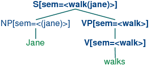

Thus, the sem value at the root node shows a semantic representation for the whole sentence, while the sem values at lower nodes show semantic representations for constituents of the sentence. So far, so good, but how do we write grammar rules which will give us this kind of result? To be more specific, suppose we have a np and vp constituents with appropriate values for their sem nodes? If you reflect on the machinery that was introduced in discussing the λ calculus, you might guess that function application will be central to composing semantic values. You will also remember that our feature-based grammar framework gives us the means to refer to variable values. Putting this together, we can postulate a rule like (16) for building the sem value of an s. (Observe that in the case where the value of sem is a variable, we omit the angle brackets.)

(16)

S[sem = <app(?vp,?subj)>] -> NP[sem=?subj] VP[sem=?vp]

(16) tells us that given some sem value ?subj for the subject np and some sem value ?vp for the vp, the sem value of the s mother is constructed by applying ?vp as a functor to ?np. From this, we can conclude that ?vp has to denote a function which has the denotation of ?np in its domain; in fact, we are going to assume that ?vp denotes a curryed characteristic function on individuals. (16) is a nice example of building semantics using the principle of compositionality: that is, the principle that the semantics of a complex expression is a function of the semantics of its parts.

To complete the grammar is very straightforward; all we require are the rules shown in (17).

(17)

VP[sem=?v] -> IV[sem=?v] NP[sem=<jane>] -> 'Jane' IV[sem=<walk>] -> 'walks'

The vp rule says that the mother's semantics is the same as the head daughter's. The two lexical rules just introduce non-logical constants to serve as the semantic values of Jane and walks respectively. This grammar can be parsed using the chart parser in parse.featurechart, and the trace in (18) shows how semantic values are derived by feature unification in the process of building a parse tree.

(18)

Predictor |> . .| S[sem='(?vp ?subj)'] -> * NP[sem=?subj] VP[sem=?vp] Scanner |[-] .| [0:1] 'Jane' Completer |[-> .| S[sem='(?vp john)'] -> NP[sem='john'] * VP[sem=?vp] Predictor |. > .| VP[sem=?v] -> * IV[sem=?v] Scanner |. [-]| [1:2] 'walks' Completer |. [-]| VP[sem='walk'] -> IV[sem='walk'] * Completer |[===]| S[sem='(walk john)'] -> NP[sem='john'] VP[sem='walk'] * Completer |[===]| [INIT] -> S *

>>> grammar = nltk.data.load('grammars/sem1.fcfg')
>>> result  = nltk.sem.text_interpret(['a dog barks'], grammar, beta_reduce=0)
>>> (syntree, semrep) = result['a dog barks'][0]
>>> print syntree
(S[sem=<exists x.(dog(x) & bark(x))>]
  (NP[sem=<\P.exists x.(dog(x) & P(x))>]
    (Det[sem=<\Q.\P.exists x.(Q(x) & P(x))>] a)
     (N[sem=<dog>] dog))
   (VP[sem=<\x.bark(x)>] (IV[sem=<\x.bark(x)>] barks)))

>>> print semrep.simplify()
exists x.(dog(x) & bark(x))

>>> grammar = nltk.data.load('grammars/sem2.fcfg')
>>> val4 = nltk.data.load('grammars/valuation1.val')
>>> dom4 = val4.domain
>>> m4 = nltk.sem.Model(dom4, val4)
>>> g = nltk.sem.Assignment(dom4)
>>> sent = 'every boy chases a girl in Noosa'
>>> result = nltk.sem.text_evaluate([sent], grammar, m4, g)
>>> for (syntree, semrep, value) in result[sent]:
...         print "'%s' is %s in Model m\n" % (semrep, value)
'all x.(boy(x) -> (exists z2.(girl(z2) & chase(x,z2)) & in(x,noosa)))' is True in Model m

'all x.(boy(x) -> (exists z2.(girl(z2) & chase(x,z2)) & in(x,noosa)))' is True in Model m

'all x.(boy(x) -> exists z3.((girl(z3) & in(z3,noosa)) & chase(x,z3)))' is False in Model m

'all x.(boy(x) -> exists z3.((girl(z3) & in(z3,noosa)) & chase(x,z3)))' is False in Model m

11.5   Case Study: Extracting Valuations from Chat-80

Building Valuation objects by hand becomes rather tedious once we consider larger examples. This raises the question of whether the relation data in a Valuation could be extracted from some pre-existing source. The corpora.chat80 module provides an example of extracting data from the Chat-80 Prolog knowledge base (which included as part of the NLTK corpora distribution).

Chat-80 data is organized into collections of clauses, where each collection functions as a table in a relational database. The predicate of the clause provides the name of the table; the first element of the tuple acts as the 'key'; and subsequent elements are further columns in the table.

In general, the name of the table provides a label for a unary relation whose extension is all the keys. For example, the table in cities.pl contains triples such as (33).

Here, 'athens' is the key, and will be mapped to a member of the unary relation city.

The other two columns in the table are mapped to binary relations, where the first argument of the relation is filled by the table key, and the second argument is filled by the data in the relevant column. Thus, in the city table illustrated by the tuple in (33), the data from the third column is extracted into a binary predicate population_of, whose extension is a set of pairs such as '(athens, 1368)'.

In order to encapsulate the results of the extraction, a class of Concepts is introduced. A Concept object has a number of attributes, in particular a prefLabel and extension, which make it easier to inspect the output of the extraction. The extension of a Concept object is incorporated into a Valuation object.

As well as deriving unary and binary relations from the Chat-80 data, we also create a set of individual constants, one for each entity in the domain. The individual constants are string-identical to the entities. For example, given a data item such as 'zloty', we add to the valuation a pair ('zloty', 'zloty'). In order to parse English sentences that refer to these entities, we also create a lexical item such as the following for each individual constant:

PropN[num=sg, sem=<\P.P(zloty)>] -> 'Zloty'

The chat80 module can be found in the corpora package. The attribute chat80.items gives us a list of Chat-80 relations:

>>> from nltk.corpus import chat80
>>> chat80.items 
 ('borders', 'circle_of_lat', 'circle_of_long', 'city', ...)

The concepts() method shows the list of Concepts that can be extracted from a chat80 relation, and we can then inspect their extensions.

>>> concepts = chat80.concepts('city')
>>> concepts
[Concept('city'), Concept('country_of'), Concept('population_of')]
>>> rel = concepts[1].extension
>>> list(rel)[:5]
[('chungking', 'china'), ('karachi', 'pakistan'),
('singapore_city', 'singapore'), ('athens', 'greece'),
('birmingham', 'united_kingdom')]

In order to convert such an extension into a valuation, we use the make_valuation() method; setting read=True creates and returns a new Valuation object which contains the results.

>>> val = nltk.corpus.chat80.make_valuation(concepts, read=True)
>>> val['city']['calcutta']
True
>>> val['country_of']['india']
{'hyderabad': True, 'delhi': True, 'bombay': True,
'madras': True, 'calcutta': True}
>>> dom = val.domain
>>> g = nltk.sem.Assignment(dom)
>>> m = nltk.sem.Model(dom, val)
>>> m.evaluate(r'\x .population_of(jakarta, x)', g)
{'533': True}

11.6   Summary

• Semantic Representations (SRs) for English are constructed using a language based on the λ-calculus, together with Boolean connectives, equality, and first-order quantifiers.
• β-reduction in the λ-calculus corresponds semantically to application of a function to an argument. Syntactically, it involves replacing a variable bound by λ in the functor with the expression that provides the argument in the function application.
• If two λ-abstracts differ only in the label of the variable bound by λ, they are said to be α equivalents. Relabeling a variable bound by a λ is called α-conversion.
• Currying of a binary function turns it into a unary function whose value is again a unary function.
• FSRL has both a syntax and a semantics. The semantics is determined by recursively evaluating expressions in a model.
• A key part of constructing a model lies in building a valuation which assigns interpretations to non-logical constants. These are interpreted as either curried characteristic functions or as individual constants.
• The interpretation of Boolean connectives is handled by the model; these are interpreted as characteristic functions.
• An open expression is an expression containing one or more free variables. Open expressions only receive an interpretation when their free variables receive values from a variable assignment.
• Quantifiers are interpreted by constructing, for a formula φ[x] open in variable x, the set of individuals which make φ[x] true when an assignment g assigns them as the value of x. The quantifier then places constraints on that set.
• A closed expression is one that has no free variables; that is, the variables are all bound. A closed sentence is true or false with respect to all variable assignments.
• Given a formula with two nested quantifiers Q₁ and Q₂, the outermost quantifier Q₁ is said to have wide scope (or scope over Q₂). English sentences are frequently ambiguous with respect to the scope of the quantifiers they contain.
• English sentences can be associated with an SR by treating sem as a feature. The sem value of a complex expressions typically involves functional application of the sem values of the component expressions.
• Model valuations need not be built by hand, but can also be extracted from relational tables, as in the Chat-80 example.

11.7   Exercises

1. ◑ Modify the sem.evaluate code so that it will give a helpful error message if an expression is not in the domain of a model's valuation function.
2. ★ Specify and implement a typed functional language with quantifiers, Boolean connectives and equality. Modify sem.evaluate to interpret expressions of this language.
3. ★ Extend the chat80 code so that it will extract data from a relational database using SQL queries.
4. ★ Taking [WarrenPereira1982] as a starting point, develop a technique for converting a natural language query into a form that can be evaluated more efficiently in a model. For example, given a query of the form '(P(x) & Q(x)', convert it to '(Q(x) & P(x)' if the extension of 'Q' is smaller than the extension of 'P'.

11.8   Further Reading

For more examples of semantic analysis with NLTK, please see the guides at http://nltk.org/doc/guides/sem.html and http://nltk.org/doc/guides/logic.html.

The use of characteristic functions for interpreting expressions of natural language was primarily due to Richard Montague. [Dowty, Wall, & Peters, 1981] gives a comprehensive and reasonably approachable introduction to Montague's grammatical framework.

A more recent and wide-reaching study of the use of a λ based approach to natural language can be found in [Carpenter, 1997].

[Heim & Kratzer, 1998] is a thorough application of formal semantics to transformational grammars in the Government-Binding model.

[Blackburn & Bos, 2005] is the first textbook devoted to computational semantics, and provides an excellent introduction to the area.