 |
OpenCV
3.0.0-dev
Open Source Computer Vision
|
 |
OpenCV
3.0.0-dev
Open Source Computer Vision
|
In this tutorial you will learn how to:
In the previous tutorial we covered two basic Morphology operations:
Based on these two we can effectuate more sophisticated transformations to our images. Here we discuss briefly 05 operations offered by OpenCV:
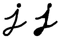
It is obtained by the erosion of an image followed by a dilation.
\[dst = open( src, element) = dilate( erode( src, element ) )\]
For instance, check out the example below. The image at the left is the original and the image at the right is the result after applying the opening transformation. We can observe that the small spaces in the corners of the letter tend to dissapear.
It is obtained by the dilation of an image followed by an erosion.
\[dst = close( src, element ) = erode( dilate( src, element ) )\]
Useful to remove small holes (dark regions).
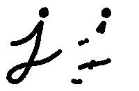
It is the difference between the dilation and the erosion of an image.
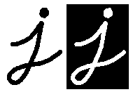
\[dst = morph_{grad}( src, element ) = dilate( src, element ) - erode( src, element )\]
It is useful for finding the outline of an object as can be seen below:

It is the difference between an input image and its opening.
\[dst = tophat( src, element ) = src - open( src, element )\]

It is the difference between the closing and its input image
\[dst = blackhat( src, element ) = close( src, element ) - src\]
This tutorial code's is shown lines below. You can also download it from here
Every time we move any slider, the user's function Morphology_Operations will be called to effectuate a new morphology operation and it will update the output image based on the current trackbar values.
We can observe that the key function to perform the morphology transformations is cv::morphologyEx . In this example we use four arguments (leaving the rest as defaults):
operation: The kind of morphology transformation to be performed. Note that we have 5 alternatives:
As you can see the values range from <2-6>, that is why we add (+2) to the values entered by the Trackbar:
After compiling the code above we can execute it giving an image path as an argument. For this tutorial we use as input the image: baboon.png:

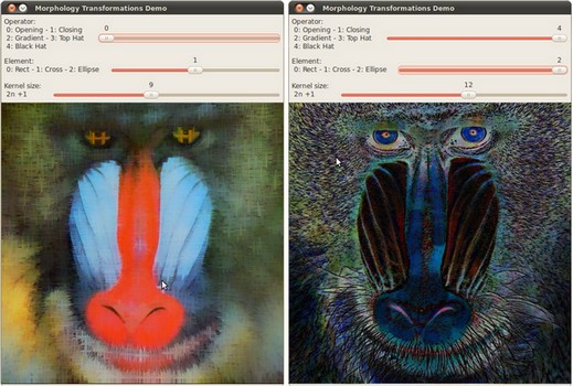
And here are two snapshots of the display window. The first picture shows the output after using the operator Opening with a cross kernel. The second picture (right side, shows the result of using a Blackhat operator with an ellipse kernel.
 1.8.9.1