

In this tutorial we formulate the learning problem for neural networks and describe some learning tasks that they can solve.
Contents:
The minimum or maximum value of the performance functional is achieved for a vector of parameters at which the performance function takes on a minimum or maximum value. Therefore, the learning problem for neural networks, formulated as a variational problem, can be reduced to a function optimization problem.
In this sense, a variational formulation for neural networks provides a direct method for solving variational problems. The universal approximation properties for the multilayer perceptron cause neural computation to be a very appropriate paradigm for the solution of these problems.
Although the performance function is multidimensional, one-dimensional optimization methods are of great importance. Indeed, one-dimensional optimization algorithms are very often used inside multidimensional optimization algorithms.
A function is said to have a relative or local minimum at some point if the function is always greater within some neighbourhood of that point. Similarly, a point is called a relative or local maximum if the function is always lesser within some neighbourhood of that point.
The function is said to have a global or absolute minimum at some point if the function is always greater within the whole domain. Similarly, a point will be a global maximum if the function is always greater within the whole domain. Finding a global optimum is, in general, a very difficult problem.
On the other hand, the tasks of maximization and minimization are trivially related to each other, since maximization of a function is equivalent to minimization of its negative, and vice versa.
In this regard, a one-dimensional optimization problem is one in which the argument which minimizes the performance function is to be found.
The necessary condition states that if the directional performance function has a relative optimum and if the derivative exists as a finite number. The condition for the optimum to be a minimum is that the second derivative is greater than zero, and vice versa.
The most elementary approach for one-dimensional optimization problems is to use a fixed step size or training rate. More sophisticated algorithms which are are widely used are the golden section method and the Brent's method. Both of the two later algorithms begin by bracketing a minimum.
The most elementary approach for such a problem is to use a fixed step size, or training rate, and move from an initial guess point in a favorable direction (positive or negative). The step size used must be small in relation to the final accuracy desired. Although this method is very simple to implement, it is not efficient in many cases.
The golden section method brackets that minimum until the distance between the two outer points in the bracket is less than a defined tolerance.
The Brent's method performs a parabolic interpolation until the distance between the two outer points defining the parabola is less than a tolerance.
As it was shown in Chapter, the learning problem for neural networks is reduced to the searching for a parameter vector at which the performance function takes a maximum or a minimum value.
The concepts of relative or local and absolute or global optima for the multidimensional case apply in the same way as for the one-dimensional case. The tasks of maximization and minimization are also trivially related here.
The necessary condition states that if the neural network is at a minimum of the performance function, then the gradient is the zero vector.
The performance function is, in general, a non linear function of the parameters. As a consequence, it is not possible to find closed training algorithms for the minima. Instead, we consider a search through the parameter space consisting of a succession of steps, or epochs.
At each epoch, the performance will increase by adjusting the neural network parameters. The change of parameters between two epochs is called the parameters increment.
In this way, to train a neural network we start with some parameters vector (often chosen at random) and we generate a sequence of parameter vectors, so that the performance function is reduced at each iteration of the algorithm. The change of performance between two epochs is called the performance improvement.
The training algorithm stops when a specified condition is satisfied. Some stopping criteria commonly used are:A stopping criterion of different nature is early stopping. This method is used in ill-posed problems in order to control the effective complexity of the neural network. Early stopping is a very common practice in neural networks and often produces good solutions to ill-possed problems.
The following figure is a state diagram of the training procedure, showing states and transitions in the training process of a neural network.
The training process is determined by the way in which the adjustment of the parameters in the neural network takes place. There are many different training algorithms, which have a variety of different computation and storage requirements. Moreover, there is not a training algorithm best suited to all locations.
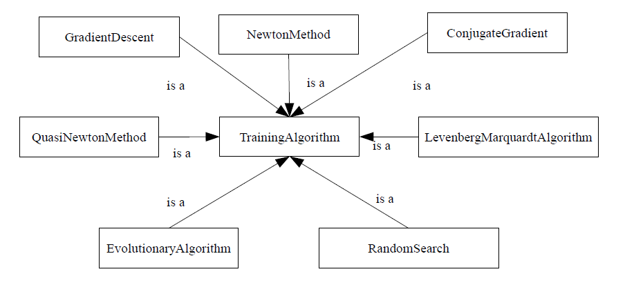
Training algorithms might require information from the performance function only, the gradient vector of the performance function or the Hessian matrix of the performance function. These methods, in turn, can perform either global or local optimization.
Zero-order training algorithms make use of the performance function only. The most significant zero-order training algorithms are stochastic, which involve randomness in the optimization process. Examples of these are random search and evolutionary algorithms or particle swarm optimization, which are global optimization methods .
First-order training algorithms use the performance function and its gradient vector. Examples of these are gradient descent methods, conjugate gradient methods, scaled conjugate gradient methods or quasi-Newton methods. Gradient descent, conjugate gradient, scaled conjugate gradient and quasi-Newton methods are local optimization methods.
Second-order training algorithms make use of the performance function, its gradient vector and its Hessian matrix. Examples for second-order methods are Newton's method and the Levenberg-Marquardt algorithm. Both of them are local optimization methods.
Most of the times, application of a single training algorithm is enough to properly train a neural network. The quasi-Newton method is in general a good choice, since it provides good training times and deals successfully with most of the performance functions. The Levenberg-Marquardt algorithm could be also recommended for small and medium-sized data modelling problems.
However, some applications might need more training effort. In that cases we can combine different algorithms in order to do our best. In problems defined by mathematical models, with constraints, etc. a single training algorithm might fail.
Therefore, for difficult problems, we can try two use two or three different training algorithms. A general strategy consists on applying three different training algorithms:
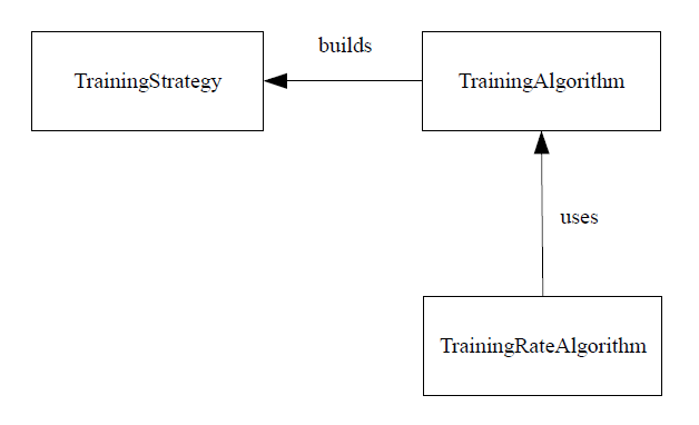
In order to construct a software model for the training strategy, a few things need to be taken into account. As we have seen, a training strategy is composed of three different training algorithms. On the other hand, some training algorithms use one-dimensional optimization for finding the optimal training rate. Therefore, the most important classes in the training strategy are:
The associations among the concepts described above are the following:
The next task is then to establish which classes are abstract and to derive the necessary concrete classes to be added. Let us then examine the classes we have so far:
The training strategy class contains:
All members are private, and must be accessed or modified by means of get and set methods, respectively.
To construct a training strategy object associated to a performance functional object we do the following:
TrainingStrategy ts(&pf);
where pf is some performance functional object.
The default training strategy consists on a main training algorithm of the quasi-Newton method type. The next sentence sets a different training strategy.
RandomSearch* rsp = new RandomSearch(&pf);
rsp->set_epochs_number(10);
ts.set_initialization_training_algorithm(rsp);

GradientDescent* gdp = new GradientDescent(&pf);
gdp->set_epochs_number(25);
ts.set_main_training_algorithm(gdp);
The most important method of a training strategy is called \lstinline"perform_training". The use is as follows:
ts.perform_training();
where ts is some training strategy object.
We can save the above object to a XML file.
ts.save("training_strategy.xml");
OpenNN Copyright © 2014 Roberto Lopez (Artelnics)