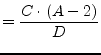
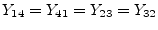
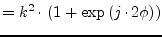
According to the port numbers in fig. 9.5
the Y-parameters of a coupler write as follows.
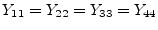 |
 |
(9.111) |
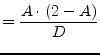
 |
 |
(9.112) |
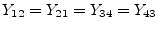
 |
 |
(9.113) |
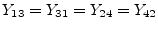
 |
 |
(9.114) |
with
 |
 |
(9.115) |
 |
 |
(9.116) |
 |
 |
(9.117) |
 |
 |
(9.118) |
whereas  denotes the coupling factor,
  the phase shift of
the coupling path and
the phase shift of
the coupling path and  the reference impedance. The coupler
can also be used as hybrid by setting
the reference impedance. The coupler
can also be used as hybrid by setting
 . For a 90 degree
hybrid, for example, set to
. For a 90 degree
hybrid, for example, set to  . Note that for most
couplers no real DC model exists. Taking the real part of the AC
matrix often leads to non-logical results. Thus, it is better to
model the coupler for DC by making a short between port 1 and port 2
and between port 3 and port 4. The rest should be an open. This
leads to the following MNA matrix.
. Note that for most
couplers no real DC model exists. Taking the real part of the AC
matrix often leads to non-logical results. Thus, it is better to
model the coupler for DC by making a short between port 1 and port 2
and between port 3 and port 4. The rest should be an open. This
leads to the following MNA matrix.
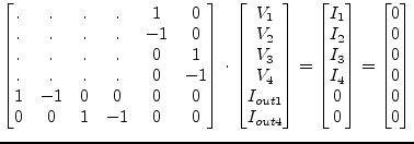 |
(9.119) |
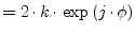
Figure 9.5:
ideal coupler device
|
|
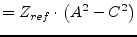
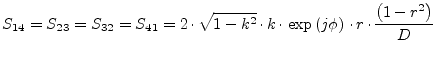
The scattering parameters of a coupler are:
 |
(9.120) |
 |
(9.121) |
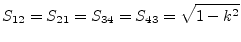 |
(9.122) |
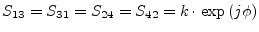 |
(9.123) |
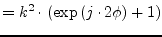
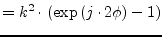
whereas denotes the coupling factor, the phase shift of
the coupling path. Extending them for an arbitrary reference
impedance , they already become quite complex:
 |
 |
(9.124) |
|
 |
(9.125) |
|
 |
(9.126) |
|
 |
(9.127) |
|
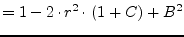 |
(9.128) |
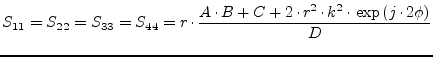 |
(9.129) |
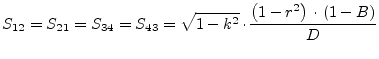 |
(9.130) |
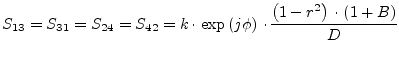 |
(9.131) |
 |
(9.132) |
An ideal coupler is noise free.
This document was generated by Stefan Jahn on 2007-12-30 using latex2html.
![\includegraphics[width=4cm]{coupler}](img1032.png)