Graph Structures¶

Debugging or profiling code written in Theano is not that simple if you do not know what goes on under the hood. This chapter is meant to introduce you to a required minimum of the inner workings of Theano.

The first step in writing Theano code is to write down all mathematical relations using symbolic placeholders (variables). When writing down these expressions you use operations like +, -, **, sum(), tanh(). All these are represented internally as ops. An op represents a certain computation on some type of inputs producing some type of output. You can see it as a function definition in most programming languages.

Theano represents symbolic mathematical computations as graphs. These graphs are composed of interconnected Apply, Variable and Op nodes. Apply node represents the application of an op to some variables. It is important to draw the difference between the definition of a computation represented by an op and its application to some actual data which is represented by the apply node. Furthermore, data types are represented by Type instances. Here is a piece of code and a diagram showing the structure built by that piece of code. This should help you understand how these pieces fit together:

Code

import theano.tensor as T

x = T.dmatrix('x')
y = T.dmatrix('y')
z = x + y

Diagram

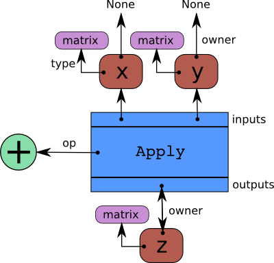
Arrows represent references to the Python objects pointed at. The blue box is an Apply node. Red boxes are Variable nodes. Green circles are Ops. Purple boxes are Types.

When we create Variables and then Apply Ops to them to make more Variables, we build a bi-partite, directed, acyclic graph. Variables point to the Apply nodes representing the function application producing them via their owner field. These Apply nodes point in turn to their input and output Variables via their inputs and outputs fields. (Apply instances also contain a list of references to their outputs, but those pointers don’t count in this graph.)

The owner field of both x and y point to None because they are not the result of another computation. If one of them was the result of another computation, it’s owner field would point to another blue box like z does, and so on.

Note that the Apply instance’s outputs points to z, and z.owner points back to the Apply instance.

Traversing the graph¶

The graph can be traversed starting from outputs (the result of some computation) down to its inputs using the owner field. Take for example the following code:

>>> import theano
>>> x = theano.tensor.dmatrix('x')
>>> y = x * 2.

If you enter type(y.owner) you get <class 'theano.gof.graph.Apply'>, which is the apply node that connects the op and the inputs to get this output. You can now print the name of the op that is applied to get y:

>>> y.owner.op.name
'Elemwise{mul,no_inplace}'

Hence, an elementwise multiplication is used to compute y. This multiplication is done between the inputs:

>>> len(y.owner.inputs)
2
>>> y.owner.inputs[0]
x
>>> y.owner.inputs[1]
InplaceDimShuffle{x,x}.0

Note that the second input is not 2 as we would have expected. This is because 2 was first broadcasted to a matrix of same shape as x. This is done by using the op DimShuffle :

>>> type(y.owner.inputs[1])
<class 'theano.tensor.var.TensorVariable'>
>>> type(y.owner.inputs[1].owner)
<class 'theano.gof.graph.Apply'>
>>> y.owner.inputs[1].owner.op 
<theano.tensor.elemwise.DimShuffle object at 0x106fcaf10>
>>> y.owner.inputs[1].owner.inputs
[TensorConstant{2.0}]

Starting from this graph structure it is easier to understand how automatic differentiation proceeds and how the symbolic relations can be optimized for performance or stability.

Graph Structures¶

The following section outlines each type of structure that may be used in a Theano-built computation graph. The following structures are explained: Apply, Constant, Op, Variable and Type.

Apply¶

An Apply node is a type of internal node used to represent a computation graph in Theano. Unlike Variable nodes, Apply nodes are usually not manipulated directly by the end user. They may be accessed via a Variable’s owner field.

An Apply node is typically an instance of the Apply class. It represents the application of an Op on one or more inputs, where each input is a Variable. By convention, each Op is responsible for knowing how to build an Apply node from a list of inputs. Therefore, an Apply node may be obtained from an Op and a list of inputs by calling Op.make_node(*inputs).

Comparing with the Python language, an Apply node is Theano’s version of a function call whereas an Op is Theano’s version of a function definition.

An Apply instance has three important fields:

op: An Op that determines the function/transformation being applied here.
inputs: A list of Variables that represent the arguments of the function.
outputs: A list of Variables that represent the return values of the function.

An Apply instance can be created by calling gof.Apply(op, inputs, outputs).

Op¶

An Op in Theano defines a certain computation on some types of inputs, producing some types of outputs. It is equivalent to a function definition in most programming languages. From a list of input Variables and an Op, you can build an Apply node representing the application of the Op to the inputs.

It is important to understand the distinction between an Op (the definition of a function) and an Apply node (the application of a function). If you were to interpret the Python language using Theano’s structures, code going like def f(x): ... would produce an Op for f whereas code like a = f(x) or g(f(4), 5) would produce an Apply node involving the f Op.

Type¶

A Type in Theano represents a set of constraints on potential data objects. These constraints allow Theano to tailor C code to handle them and to statically optimize the computation graph. For instance, the irow type in the theano.tensor package gives the following constraints on the data the Variables of type irow may contain:

Must be an instance of numpy.ndarray: isinstance(x, numpy.ndarray)
Must be an array of 32-bit integers: str(x.dtype) == 'int32'
Must have a shape of 1xN: len(x.shape) == 2 and x.shape[0] == 1

Knowing these restrictions, Theano may generate C code for addition, etc. that declares the right data types and that contains the right number of loops over the dimensions.

Note that a Theano Type is not equivalent to a Python type or class. Indeed, in Theano, irow and dmatrix both use numpy.ndarray as the underlying type for doing computations and storing data, yet they are different Theano Types. Indeed, the constraints set by dmatrix are:

Must be an instance of numpy.ndarray: isinstance(x, numpy.ndarray)
Must be an array of 64-bit floating point numbers: str(x.dtype) == 'float64'
Must have a shape of MxN, no restriction on M or N: len(x.shape) == 2

These restrictions are different from those of irow which are listed above.

There are cases in which a Type can fully correspond to a Python type, such as the double Type we will define here, which corresponds to Python’s float. But, it’s good to know that this is not necessarily the case. Unless specified otherwise, when we say “Type” we mean a Theano Type.

Variable¶

A Variable is the main data structure you work with when using Theano. The symbolic inputs that you operate on are Variables and what you get from applying various Ops to these inputs are also Variables. For example, when I type

>>> import theano
>>> x = theano.tensor.ivector()
>>> y = -x

x and y are both Variables, i.e. instances of the Variable class. The Type of both x and y is theano.tensor.ivector.

Unlike x, y is a Variable produced by a computation (in this case, it is the negation of x). y is the Variable corresponding to the output of the computation, while x is the Variable corresponding to its input. The computation itself is represented by another type of node, an Apply node, and may be accessed through y.owner.

More specifically, a Variable is a basic structure in Theano that represents a datum at a certain point in computation. It is typically an instance of the class Variable or one of its subclasses.

A Variable r contains four important fields:

type: a Type defining the kind of value this Variable can hold in computation.
owner: this is either None or an Apply node of which the Variable is an output.
index: the integer such that owner.outputs[index] is r (ignored if owner is None)
name: a string to use in pretty-printing and debugging.

Variable has one special subclass: Constant.

Constant¶

A Constant is a Variable with one extra field, data (only settable once). When used in a computation graph as the input of an Op application, it is assumed that said input will always take the value contained in the constant’s data field. Furthermore, it is assumed that the Op will not under any circumstances modify the input. This means that a constant is eligible to participate in numerous optimizations: constant inlining in C code, constant folding, etc.

A constant does not need to be specified in a function‘s list of inputs. In fact, doing so will raise an exception.

Graph Structures Extension¶

When we start the compilation of a Theano function, we compute some extra information. This section describes a portion of the information that is made available. Not everything is described, so email theano-dev if you need something that is missing.

The graph gets cloned at the start of compilation, so modifications done during compilation won’t affect the user graph.

Each variable receives a new field called clients. It is a list with references to every place in the graph where this variable is used. If its length is 0, it means the variable isn’t used. Each place where it is used is described by a tuple of 2 elements. There are two types of pairs:

The first element is an Apply node.
The first element is the string “output”. It means the function outputs this variable.

In both types of pairs, the second element of the tuple is an index, such that: var.clients[*][0].inputs[index] or fgraph.outputs[index] is that variable.

>>> import theano
>>> v = theano.tensor.vector()
>>> f = theano.function([v], (v+1).sum())
>>> theano.printing.debugprint(f)
Sum{acc_dtype=float64} [id A] ''   1
 |Elemwise{add,no_inplace} [id B] ''   0
   |TensorConstant{(1,) of 1.0} [id C]
   |<TensorType(float64, vector)> [id D]
>>> # Sorted list of all nodes in the compiled graph.
>>> topo = f.maker.fgraph.toposort()
>>> topo[0].outputs[0].clients
[(Sum{acc_dtype=float64}(Elemwise{add,no_inplace}.0), 0)]
>>> topo[1].outputs[0].clients
[('output', 0)]

>>> # An internal variable
>>> var = topo[0].outputs[0]
>>> client = var.clients[0]
>>> client
(Sum{acc_dtype=float64}(Elemwise{add,no_inplace}.0), 0)
>>> type(client[0])
<class 'theano.gof.graph.Apply'>
>>> assert client[0].inputs[client[1]] is var

>>> # An output of the graph
>>> var = topo[1].outputs[0]
>>> client = var.clients[0]
>>> client
('output', 0)
>>> assert f.maker.fgraph.outputs[client[1]] is var

Automatic Differentiation¶

Having the graph structure, computing automatic differentiation is simple. The only thing tensor.grad() has to do is to traverse the graph from the outputs back towards the inputs through all apply nodes (apply nodes are those that define which computations the graph does). For each such apply node, its op defines how to compute the gradient of the node’s outputs with respect to its inputs. Note that if an op does not provide this information, it is assumed that the gradient is not defined. Using the chain rule these gradients can be composed in order to obtain the expression of the gradient of the graph’s output with respect to the graph’s inputs.

A following section of this tutorial will examine the topic of differentiation in greater detail.

Optimizations¶

When compiling a Theano function, what you give to the theano.function is actually a graph (starting from the output variables you can traverse the graph up to the input variables). While this graph structure shows how to compute the output from the input, it also offers the possibility to improve the way this computation is carried out. The way optimizations work in Theano is by identifying and replacing certain patterns in the graph with other specialized patterns that produce the same results but are either faster or more stable. Optimizations can also detect identical subgraphs and ensure that the same values are not computed twice or reformulate parts of the graph to a GPU specific version.

For example, one (simple) optimization that Theano uses is to replace the pattern $\frac{xy}{y}$ by x.

Further information regarding the optimization process and the specific optimizations that are applicable is respectively available in the library and on the entrance page of the documentation.

Example

Symbolic programming involves a change of paradigm: it will become clearer as we apply it. Consider the following example of optimization:

>>> import theano
>>> a = theano.tensor.vector("a")      # declare symbolic variable
>>> b = a + a ** 10                    # build symbolic expression
>>> f = theano.function([a], b)        # compile function
>>> print(f([0, 1, 2]))                # prints `array([0,2,1026])`
[    0.     2.  1026.]
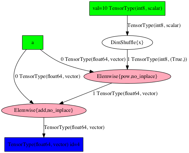
>>> theano.printing.pydotprint(b, outfile="./pics/symbolic_graph_unopt.png", var_with_name_simple=True)  
The output file is available at ./pics/symbolic_graph_unopt.png
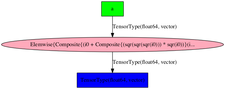
>>> theano.printing.pydotprint(f, outfile="./pics/symbolic_graph_opt.png", var_with_name_simple=True)  
The output file is available at ./pics/symbolic_graph_opt.png

We used theano.printing.pydotprint() to visualize the optimized graph (right), which is much more compact than the unoptimized graph (left).

Unoptimized graph		Optimized graph