Concepts¶

In this section we summarize the key concepts of Kafka Streams. For more detailed information please refer to Architecture and the Developer Guide.

Kafka 101¶

Kafka Streams is, by deliberate design, tightly integrated with Apache Kafka: it uses Kafka as its internal messaging layer. As such it is important to familiarize yourself with the key concepts of Kafka, too, notably the sections 1. Getting Started and 4. Design in the Kafka documentation. In particular you should understand:

The who’s who: Kafka distinguishes producers, consumers, and brokers. In short, producers publish data to Kafka brokers, and consumers read published data from Kafka brokers. Producers and consumers are totally decoupled. A Kafka cluster consists of one or more brokers.
The data: Data is stored in topics. The topic is the most important abstraction provided by Kafka: it is a category or feed name to which data is published by producers. Every topic in Kafka is split into one or more partitions, which are replicated across Kafka brokers for fault tolerance.
Parallelism: Partitions of Kafka topics, and especially their number for a given topic, are also the main factor that determines the parallelism of Kafka with regards to reading and writing data. Because of their tight integration the parallelism of Kafka Streams is heavily influenced by and depending on Kafka’s parallelism.

Stream¶

A stream is the most important abstraction provided by Kafka Streams: it represents an unbounded, continuously updating data set, where unbounded means “of unknown or of unlimited size”. A stream is an ordered, replayable, and fault-tolerant sequence of immutable data records, where a data record is defined as a key-value pair.

Stream Processing Application¶

A stream processing application is any program that makes use of the Kafka Streams library. In practice, this means it is probably “your” Java application. It may define its computational logic through one or more processor topologies (see next section).

Processor Topology¶

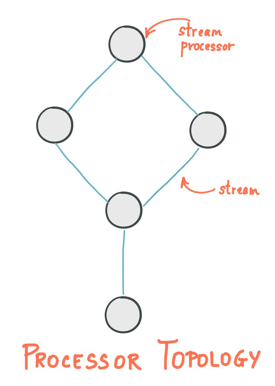
A processor topology or simply topology defines the computational logic of the data processing that needs to be performed by a stream processing application. A topology is a graph of stream processors (nodes) that are connected by streams (edges). Developers can define topologies either via the low-level Processor API or via the Kafka Streams DSL, which builds on top of the former.

../_images/streams-concepts-topology.jpg

The Architecture documentation describes topologies in more detail.

Stream Processor¶

A stream processor is a node in the processor topology as shown in the diagram of section Processor Topology). It represents a processing step in a topology, i.e. it is used to transform data in streams. Standard operations such as map, filter, join, and aggregations are examples of stream processors that are available in Kafka Streams out of the box. A stream processor receives one input record at a time from its upstream processors in the topology, applies its operation to it, and may subsequently produce one or more output records to its downstream processors.

Kafka Streams provides two ways to define stream processors:

The Kafka Streams DSL provides the most common data transformation operations such as map and filter so you don’t have to implement these stream processors from scratch.
The low-level Processor API allows developers to define and connect custom processors as well as to interact with state stores.

Time¶

A critical aspect in stream processing is the the notion of time, and how it is modeled and integrated. For example, some operations such as Windowing are defined based on time boundaries.

Common notions of time in streams are:

Event-time: The point in time when an event or data record occurred, i.e. was originally created “by the source”. Achieving event-time semantics typically requires embedding timestamps in the data records at the time a data record is being produced.
- Example: If the event is a geo-location change reported by a GPS sensor in a car, then the associated event-time would be the time when the GPS sensor captured the location change.
Processing-time: The point in time when the event or data record happens to be processed by the stream processing application, i.e. when the record is being consumed. The processing-time may be milliseconds, hours, or days etc. later than the original event-time.
- Example: Imagine an analytics application that reads and processes the geo-location data reported from car sensors to present it to a fleet management dashboard. Here, processing-time in the analytics application might be milliseconds or seconds (e.g. for real-time pipelines based on Apache Kafka and Kafka Streams) or hours (e.g. for batch pipelines based on Apache Hadoop or Apache Spark) after event-time.
Ingestion-time: The point in time when an event or data record is stored in a topic partition by a Kafka broker. Ingestion-time is similar to event-time, as a timestamp gets embedded in the data record itself. The difference is, that the timestamp is generated when the record is appended to the target topic by the Kafka broker, not when the record is created “at the source”. Ingestion-time may approximate event-time reasonably well if we assume that the time difference between creation of the record and its ingestion into Kafka is sufficiently small, where “sufficiently” depends on the specific use case. Thus, ingestion-time may be a reasonable alternative for use cases where event-time semantics are not possible, e.g. because the data producers don’t embed timestamps (e.g. older versions of Kafka’s Java producer client) or the producer cannot assign timestamps directly (e.g., it does not have access to a local clock).

The choice between event-time and ingestion-time is actually done through the configuration of Kafka (not Kafka Streams): From Kafka 0.10.x onwards, timestamps are automatically embedded into Kafka messages. Depending on Kafka’s configuration these timestamps represent event-time or ingestion-time. The respective Kafka configuration setting can be specified on the broker level or per topic. The default timestamp extractor in Kafka Streams will retrieve these embedded timestamps as-is. Hence, the effective time semantics of your application depend on the effective Kafka configuration for these embedded timestamps. See timestamp extractors for detailed information.

Kafka Streams assigns a timestamp to every data record via so-called timestamp extractors. These per-record timestamps describe the progress of a stream with regards to time (although records may be out-of-order within the stream) and are leveraged by time-dependent operations such as joins. They are also used to synchronize multiple input streams within the same application.

Concrete implementations of timestamp extractors may retrieve or compute timestamps based on the actual contents of data records such as an embedded timestamp field to provide event-time or ingestion-time semantics, or use any other approach such as returning the current wall-clock time at the time of processing, thereby yielding processing-time semantics to stream processing applications. Developers can thus enforce different notions/semantics of time depending on their business needs.

Finally, whenever a Kafka Streams application writes records to Kafka, then it will also assign timestamps to these new records. The way the timestamps are assigned depends on the context:

When new output records are generated via processing some input record, for example, context.forward() triggered in the process() function call, output record timestamps are inherited from input record timestamps directly.
When new output records are generated via periodic functions such as punctuate(), the output record timestamp is defined as the current internal time (obtained through context.timestamp()) of the stream task. Note that punctuate() is triggered data-driven and not based on wall-clock time (c.f. Developer Guide).
For aggregations, the timestamp of a resulting aggregate update record will be that of the latest input record that triggered the update.

Attention

Be aware that ingestion-time in Kafka Streams is used slightly different as in other stream processing systems. Ingestion-time could mean the time when a record is fetched by a stream processing application’s source operator. In Kafka Streams, ingestion-time refers to the time when a record was appended to a Kafka topic partition.

Tip

Know your time: When working with time you should also make sure that additional aspects of time such as time zones and calendars are correctly synchronized – or at least understood and traced – throughout your stream data pipelines. It often helps, for example, to agree on specifying time information in UTC or in Unix time (such as seconds since the epoch). You should also not mix topics with different time semantics.

Stateful Stream Processing¶

Some stream processing applications don’t require state, which means the processing of a message is independent from the processing of all other messages. If you only need to transform one message at a time, or filter out messages based on some condition, the topology defined in your stream processing application can be simple.

However, being able to maintain state opens up many possibilities for sophisticated stream processing applications: you can join input streams, or group and aggregate data records. Many such stateful operators are provided by the Kafka Streams DSL.

Duality of Streams and Tables¶

Before we discuss concepts such as aggregations in Kafka Streams we must first introduce tables, and most importantly the relationship between tables and streams: the so-called stream-table duality. Essentially, this duality means that a stream can be viewed as a table, and vice versa. Kafka’s log compaction feature, for example, exploits this duality.

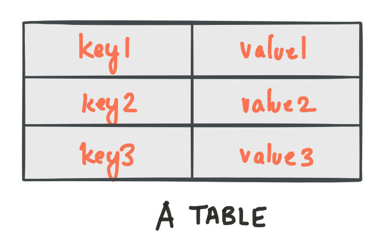
A simple form of a table is a collection of key-value pairs, also called a map or associative array.

Note

We intentionally keep this section simple and thus skip the discussion of compound keys, multisets, and so on.

Such a table may look as follows:

The stream-table duality describes the close relationship between streams and tables.

Stream as Table: A stream can be considered a changelog of a table, where each data record in the stream captures a state change of the table. A stream is thus a table in disguise, and it can be easily turned into a “real” table by replaying the changelog from beginning to end to reconstruct the table. Similarly, in a more general analogy, aggregating data records in a stream – such as computing the total number of pageviews by user from a stream of pageview events – will return a table (here with the key and the value being the user and its corresponding pageview count, respectively).
Table as Stream: A table can be considered a snapshot, at a point in time, of the latest value for each key in a stream (a stream’s data records are key-value pairs). A table is thus a stream in disguise, and it can be easily turned into a “real” stream by iterating over each key-value entry in the table.

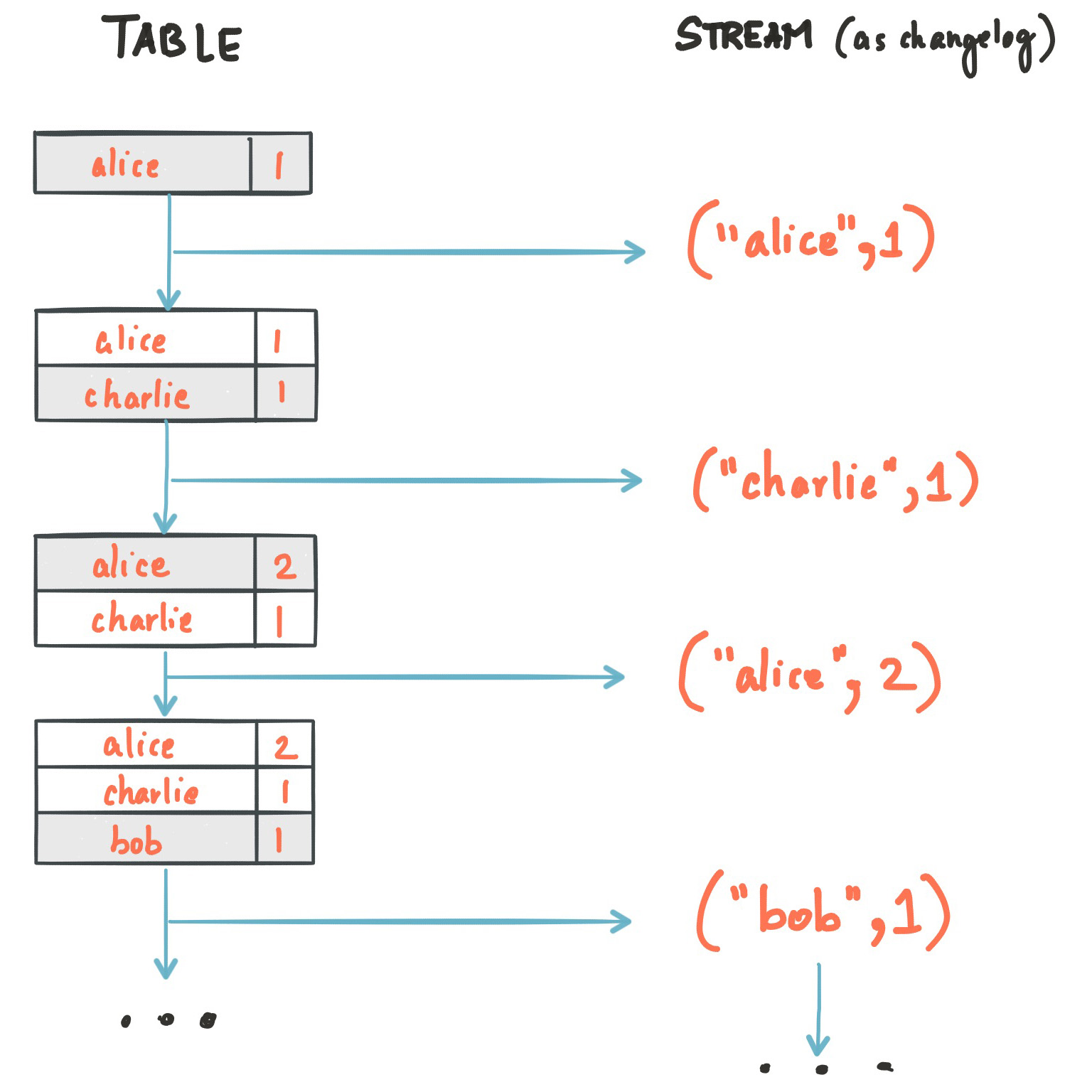
Let’s illustrate this with an example. Imagine a table that tracks the total number of pageviews by user (first column of diagram below). Over time, whenever a new pageview event is processed, the state of the table is updated accordingly. Here, the state changes between different points in time – and different revisions of the table – can be represented as a changelog stream (second column).

Interestingly, because of the stream-table duality, the same stream can be used to reconstruct the original table (third column):

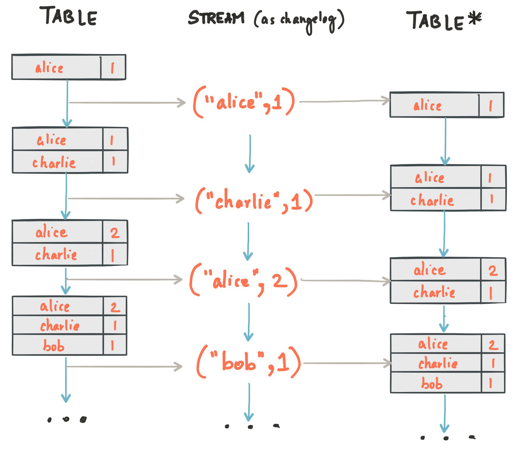
The same mechanism is used, for example, to replicate databases via change data capture (CDC) and, within Kafka Streams, to replicate its so-called state stores across machines for fault-tolerance. The stream-table duality is such an important concept that Kafka Streams models it explicitly via the KStream and KTable interfaces, which we describe in the next sections.

KStream (record stream)¶

Note

Only the Kafka Streams DSL has the notion of a KStream.

A KStream is an abstraction of a record stream, where each data record represents a self-contained datum in the unbounded data set. Using the table analogy, data records in a record stream are always interpreted as “inserts” – think: append-only ledger – because no record replaces an existing row with the same key. Examples are a credit card transaction, a page view event, or a server log entry.

To illustrate, let’s imagine the following two data records are being sent to the stream:

("alice", 1) --> ("alice", 3)

If your stream processing application were to sum the values per user, it would return 4 for alice. Why? Because the second data record would not be considered an update of the previous record. Compare this behavior of KStream to KTable below, which would return 3 for alice.

KTable (changelog stream)¶

Note

Only the Kafka Streams DSL has the notion of a KTable.

A KTable is an abstraction of a changelog stream, where each data record represents an update. More precisely, the value in a data record is considered to be an update of the last value for the same record key, if any (if a corresponding key doesn’t exist yet, the update will be considered a create). Using the table analogy, a data record in a changelog stream is interpreted as an update because any existing row with the same key is overwritten.

To illustrate, let’s imagine the following two data records are being sent to the stream:

("alice", 1) --> ("alice", 3)

If your stream processing application were to sum the values per user, it would return 3 for alice. Why? Because the second data record would be considered an update of the previous record. Compare this behavior of KTable with the illustration for KStream above, which would return 4 for alice.

Note

Effects of Kafka’s log compaction: Another way of thinking about KStream and KTable is as follows: If you were to store a KTable into a Kafka topic, you’d probably want to enable Kafka’s log compaction feature, e.g. to save storage space.

However, it would not be safe to enable log compaction in the case of a KStream because, as soon as log compaction would begin purging older data records of the same key, it would break the semantics of the data. To pick up the illustration example again, you’d suddenly get a 3 for alice instead of a 4 because log compaction would have removed the ("alice", 1) data record. Hence log compaction is perfectly safe for a KTable (changelog stream) but it is a mistake for a KStream (record stream).

We have already seen an example of a changelog stream in the section Duality of Streams and Tables. Another example are change data capture (CDC) records in the changelog of a relational database, representing which row in a database table was inserted, updated, or deleted.

KTable also provides an ability to look up current values of data records by keys. This table-lookup functionality is available through join operations (see also Joining Streams in the Developer Guide).

Windowing¶

A stream processor may need to divide data records into time buckets, i.e. to window the stream by time. This is usually needed for for join and aggregation operations, etc. Windowed stream buckets can be maintained in the processor’s local state.

Windowing operations are available in the Kafka Streams DSL, where users can specify a retention period for the window. This allows Kafka Streams to retain old window buckets for a period of time in order to wait for the late arrival of records whose timestamps fall within the window interval. If a record arrives after the retention period has passed, the record cannot be processed and is dropped.

Late-arriving records are always possible in real-time data streams. However, it depends on the effective time semantics how late records are handled. Using processing-time, the semantics are “when the data is being processed”, which means that the notion of late records is not applicable as, by definition, no record can be late. Hence, late-arriving records only really can be considered as such (i.e. as arriving “late”) for event-time or ingestion-time semantics. In both cases, Kafka Streams is able to properly handle late-arriving records.

Joins¶

A join operation merges two streams based on the keys of their data records, and yields a new stream. A join over record streams usually needs to be performed on a windowing basis because otherwise the number of records that must be maintained for performing the join may grow indefinitely.

The join operations available in the Kafka Streams DSL differ based on which kinds of streams are being joined (e.g. KStream-KStream join versus KStream-KTable join).

Aggregations¶

An aggregation operation takes one input stream, and yields a new stream by combining multiple input records into a single output record. Examples of aggregations are computing counts or sum. An aggregation over record streams usually needs to be performed on a windowing basis because otherwise the number of records that must be maintained for performing the aggregation may grow indefinitely.

In the Kafka Streams DSL, an input stream of an aggregation can be a KStream or a KTable, but the output stream will always be a KTable. This allows Kafka Streams to update an aggregate value upon the late arrival of further records after the value was produced and emitted. When such late arrival happens, the aggregating KStream or KTable simply emits a new aggregate value. Because the output is a KTable, the new value is considered to overwrite the old value with the same key in subsequent processing steps.