Concepts¶

In this section we summarize the key concepts of Kafka Streams. For more detailed information please refer to Architecture and the Developer Guide.

Table of Contents

Kafka 101 ¶

Kafka Streams is, by deliberate design, tightly integrated with Apache Kafka: many capabilities of Kafka Streams such as its stateful processing features, its fault tolerance, and its processing guarantees are built on top of functionality provided by Kafka’s storage and messaging layer. It is therefore important to familiarize yourself with the key concepts of Kafka, notably the sections Getting Started and Design in the Kafka documentation. In particular you should understand:

The who’s who: Kafka distinguishes producers, consumers, and brokers. In short, producers publish data to Kafka brokers, and consumers read published data from Kafka brokers. Producers and consumers are totally decoupled, and both run outside the Kafka brokers in the perimeter of a Kafka cluster. A Kafka cluster consists of one or more brokers. An application that uses the Kafka Streams API acts as both a producer and a consumer.
The data: Data is stored in topics. The topic is the most important abstraction provided by Kafka: it is a category or feed name to which data is published by producers. Every topic in Kafka is split into one or more partitions. Kafka partitions data for storing, transporting, and replicating it. Kafka Streams partitions data for processing it. In both cases, this partitioning enables elasticity, scalability, high performance, and fault tolerance.
Parallelism: Partitions of Kafka topics, and especially their number for a given topic, are also the main factor that determines the parallelism of Kafka with regards to reading and writing data. Because of the tight integration with Kafka, the parallelism of an application that uses the Kafka Streams API is primarily depending on Kafka’s parallelism.

Stream ¶

A stream is the most important abstraction provided by Kafka Streams: it represents an unbounded, continuously updating data set, where unbounded means “of unknown or of unlimited size”. Just like a topic in Kafka, a stream in the Kafka Streams API consists of one or more stream partitions.

A stream partition is an, ordered, replayable, and fault-tolerant sequence of immutable data records, where a data record is defined as a key-value pair.

Stream Processing Application ¶

A stream processing application is any program that makes use of the Kafka Streams library. In practice, this means it is probably “your” application. It may define its computational logic through one or more processor topologies.

An application instance is any running instance or “copy” of your application. Application instances are the primary means to elasticly scale and parallelize your application, and they also contribute to making it fault-tolerant. For example, you may need the power of ten machines to handle the incoming data load of your application; here, you could opt to run ten instances of your application, one on each machine, and these instances would automatically collaborate on the data processing – even as new instances/machines are added or existing ones removed during live operation.

Processor Topology ¶

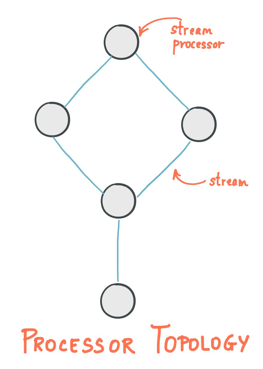
A processor topology or simply topology defines the computational logic of the data processing that needs to be performed by a stream processing application. A topology is a graph of stream processors (nodes) that are connected by streams (edges). Developers can define topologies either via the low-level Processor API or via the Kafka Streams DSL, which builds on top of the former.

../_images/streams-concepts-topology.jpg

The Architecture documentation describes topologies in more detail.

Stream Processor ¶

A stream processor is a node in the processor topology as shown in the diagram of section Processor Topology. It represents a processing step in a topology, i.e. it is used to transform data. Standard operations such as map or filter, joins, and aggregations are examples of stream processors that are available in Kafka Streams out of the box. A stream processor receives one input record at a time from its upstream processors in the topology, applies its operation to it, and may subsequently produce one or more output records to its downstream processors.

Kafka Streams provides two APIs to define stream processors:

The declarative, functional DSL is the recommended API for most users – and notably for starters – because most data processing use cases can be expressed in just a few lines of DSL code. Here, you typically use built-in operations such as map and filter.
The imperative, lower-level Processor API provides you with even more flexibility than the DSL but at the expense of requiring more manual coding work. Here, you can define and connect custom processors as well as directly interact with state stores.

Stateful Stream Processing ¶

Some stream processing applications don’t require state – they are stateless – which means the processing of a message is independent from the processing of other messages. Examples are when you only need to transform one message at a time, or filter out messages based on some condition.

In practice, however, most applications require state – they are stateful – in order to work correctly, and this state must be managed in a fault-tolerant manner. Your application is stateful whenever, for example, it needs to join, aggregate, or window its input data. Kafka Streams provides your application with powerful, elastic, highly scalable, and fault-tolerant stateful processing capabilities.

Duality of Streams and Tables ¶

When implementing stream processing use cases in practice, you typically need both streams and also databases. An example use case that is very common in practice is an e-commerce application that enriches an incoming stream of customer transactions with the latest customer information from a database table. In other words, streams are everywhere, but databases are everywhere, too.

Any stream processing technology must therefore provide first-class support for streams and tables. Kafka’s Streams API provides such functionality through its core abstractions for streams and tables, which we will talk about in a minute. Now, an interesting observation is that there is actually a close relationship between streams and tables, the so-called stream-table duality. And Kafka exploits this duality in many ways: for example, to make your applications elastic, to support fault-tolerant stateful processing, or to run interactive queries against your application’s latest processing results. And, beyond its internal usage, the Kafka Streams API also allows developers to exploit this duality in their own applications.

Before we discuss concepts such as aggregations in Kafka Streams we must first introduce tables in more detail, and talk about the aforementioned stream-table duality. Essentially, this duality means that a stream can be viewed as a table, and a table can be viewed as a stream.

Note

We intentionally keep the following explanations simple and thus skip the discussion of compound keys, multisets, and so on.

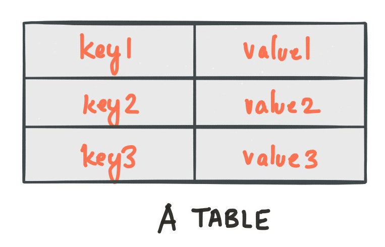
A simple form of a table is a collection of key-value pairs, also called a map or associative array. Such a table may look as follows:

The stream-table duality describes the close relationship between streams and tables.

Stream as Table: A stream can be considered a changelog of a table, where each data record in the stream captures a state change of the table. A stream is thus a table in disguise, and it can be easily turned into a “real” table by replaying the changelog from beginning to end to reconstruct the table. Similarly, aggregating data records in a stream will return a table. For example, we could compute the total number of pageviews by user from an input stream of pageview events, and the result would be a table, with the table key being the user and the value being the corresponding pageview count.
Table as Stream: A table can be considered a snapshot, at a point in time, of the latest value for each key in a stream (a stream’s data records are key-value pairs). A table is thus a stream in disguise, and it can be easily turned into a “real” stream by iterating over each key-value entry in the table.

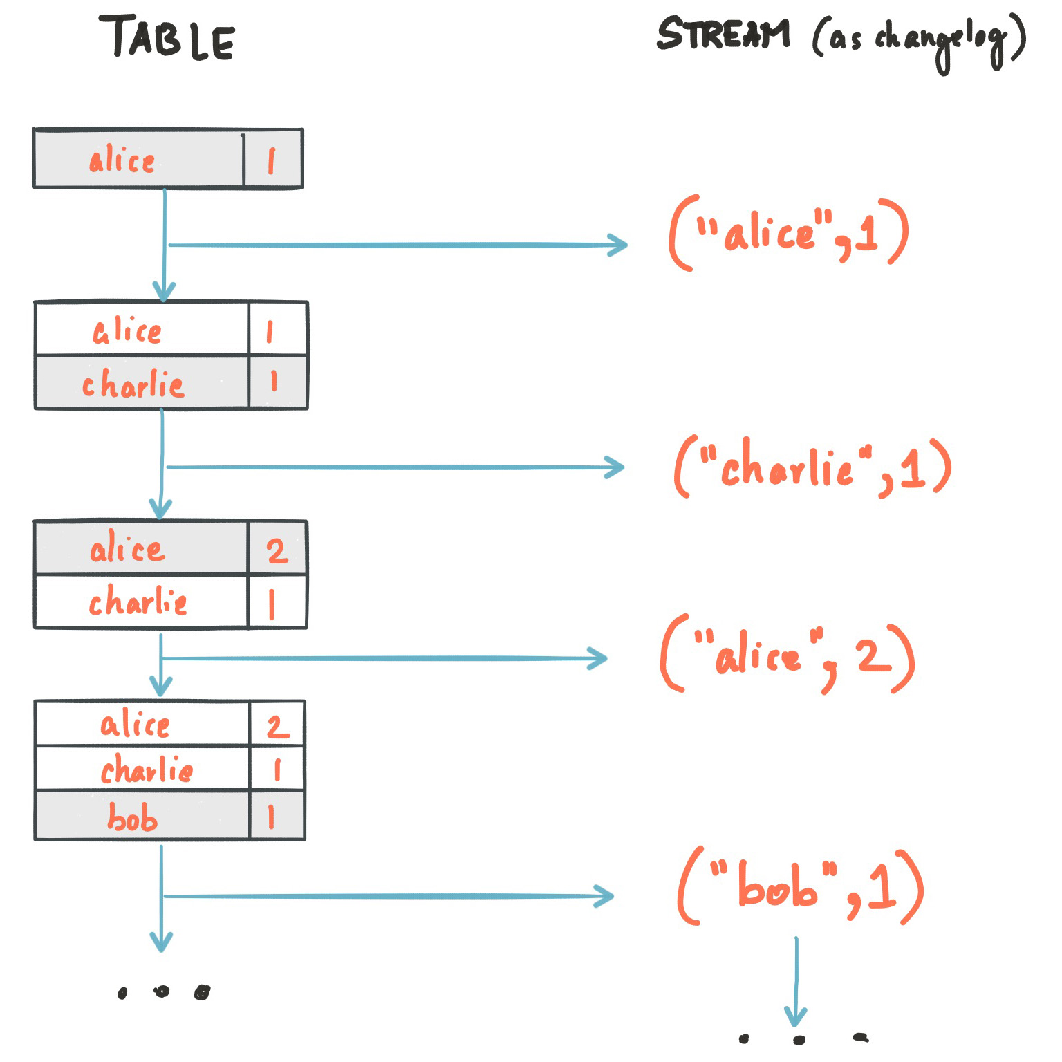
Let’s illustrate this with an example. Imagine a table that tracks the total number of pageviews by user (first column of diagram below). Over time, whenever a new pageview event is processed, the state of the table is updated accordingly. Here, the state changes between different points in time – and different revisions of the table – can be represented as a changelog stream (second column).

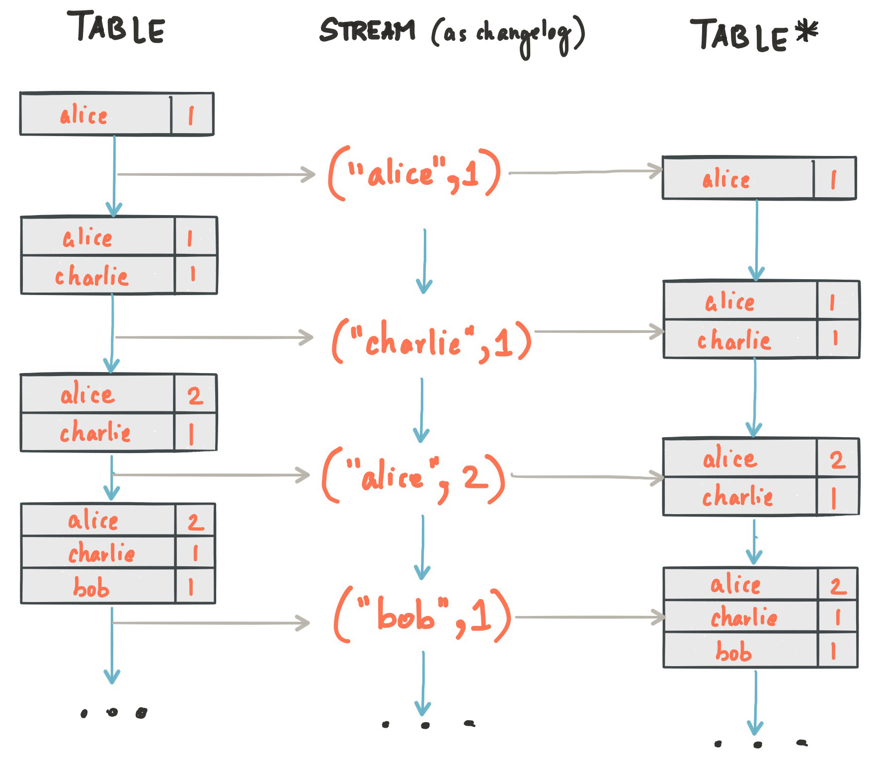
Because of the stream-table duality, the same stream can be used to reconstruct the original table (third column):

The same mechanism is used, for example, to replicate databases via change data capture (CDC) and, within Kafka Streams, to replicate its so-called state stores across machines for fault tolerance. The stream-table duality is such an important concept for stream processing applications in practice that Kafka Streams models it explicitly via the KStream and KTable abstractions, which we describe in the next sections.

KStream ¶

Note

Only the Kafka Streams DSL has the notion of a KStream.

A KStream is an abstraction of a record stream, where each data record represents a self-contained datum in the unbounded data set. Using the table analogy, data records in a record stream are always interpreted as an “INSERT” – think: adding more entries to an append-only ledger – because no record replaces an existing row with the same key. Examples are a credit card transaction, a page view event, or a server log entry.

To illustrate, let’s imagine the following two data records are being sent to the stream:

("alice", 1) --> ("alice", 3)

If your stream processing application were to sum the values per user, it would return 4 for alice. Why? Because the second data record would not be considered an update of the previous record. Compare this behavior of KStream to KTable below, which would return 3 for alice.

KTable ¶

Note

Only the Kafka Streams DSL has the notion of a KTable.

A KTable is an abstraction of a changelog stream, where each data record represents an update. More precisely, the value in a data record is interpreted as an “UPDATE” of the last value for the same record key, if any (if a corresponding key doesn’t exist yet, the update will be considered an INSERT). Using the table analogy, a data record in a changelog stream is interpreted as an UPSERT aka INSERT/UPDATE because any existing row with the same key is overwritten. Also, null values are interpreted in a special way: a record with a null value represents a “DELETE” or tombstone for the record’s key.

To illustrate, let’s imagine the following two data records are being sent to the stream:

("alice", 1) --> ("alice", 3)

If your stream processing application were to sum the values per user, it would return 3 for alice. Why? Because the second data record would be considered an update of the previous record. Compare this behavior of KTable with the illustration for KStream above, which would return 4 for alice.

Note

Effects of Kafka’s log compaction: Another way of thinking about KStream and KTable is as follows: If you were to store a KTable into a Kafka topic, you’d probably want to enable Kafka’s log compaction feature, e.g. to save storage space.

However, it would not be safe to enable log compaction in the case of a KStream because, as soon as log compaction would begin purging older data records of the same key, it would break the semantics of the data. To pick up the illustration example again, you’d suddenly get a 3 for alice instead of a 4 because log compaction would have removed the ("alice", 1) data record. Hence log compaction is perfectly safe for a KTable (changelog stream) but it is a mistake for a KStream (record stream).

We have already seen an example of a changelog stream in the section Duality of Streams and Tables. Another example are change data capture (CDC) records in the changelog of a relational database, representing which row in a database table was inserted, updated, or deleted.

KTable also provides an ability to look up current values of data records by keys. This table-lookup functionality is available through join operations (see also Joining in the Developer Guide) as well as through Interactive Queries.

GlobalKTable ¶

Note

Only the Kafka Streams DSL has the notion of a GlobalKTable.

Like a KTable, a GlobalKTable is an abstraction of a changelog stream, where each data record represents an update.

A GlobalKTable differs from a KTable in the data that they are being populated with, i.e. which data from the underlying Kafka topic is being read into the respective table. Slightly simplified, imagine you have an input topic with 5 partitions. In your application, you want to read this topic into a table. Also, you want to run your application across 5 application instances for maximum parallelism.

If you read the input topic into a KTable, then the “local” KTable instance of each application instance will be populated with data from only 1 partition of the topic’s 5 partitions.
If you read the input topic into a GlobalKTable, then the local GlobalKTable instance of each application instance will be populated with data from all partitions of the topic.

GlobalKTable provides the ability to look up current values of data records by keys. This table-lookup functionality is available through join operations (see also Joining in the Developer Guide) and Interactive Queries.

Benefits of global tables:

More convenient and/or efficient joins: Notably, global tables allow you to perform star joins, they support “foreign-key” lookups (i.e., you can lookup data in the table not just by record key, but also by data in the record values), and they are more efficient when chaining multiple joins. Also, when joining against a global table, the input data does not need to be co-partitioned.
Can be used to “broadcast” information to all the running instances of your application.

Downsides of global tables:

Increased local storage consumption compared to the (partitioned) KTable because the entire topic is tracked.
Increased network and Kafka broker load compared to the (partitioned) KTable because the entire topic is read.

Time ¶

A critical aspect in stream processing is the the notion of time, and how it is modeled and integrated. For example, some operations such as Windowing are defined based on time boundaries.

Kafka Streams supports the following notions of time:

Event-time: The point in time when an event or data record occurred, i.e. was originally created “by the source”. Achieving event-time semantics typically requires embedding timestamps in the data records at the time a data record is being produced.
- Example: If the event is a geo-location change reported by a GPS sensor in a car, then the associated event-time would be the time when the GPS sensor captured the location change.
Processing-time: The point in time when the event or data record happens to be processed by the stream processing application, i.e. when the record is being consumed. The processing-time may be milliseconds, hours, or days etc. later than the original event-time.
- Example: Imagine an analytics application that reads and processes the geo-location data reported from car sensors to present it to a fleet management dashboard. Here, processing-time in the analytics application might be milliseconds or seconds (e.g. for real-time pipelines based on Apache Kafka and Kafka Streams) or hours (e.g. for batch pipelines based on Apache Hadoop or Apache Spark) after event-time.
Ingestion-time: The point in time when an event or data record is stored in a topic partition by a Kafka broker. Ingestion-time is similar to event-time, as a timestamp gets embedded in the data record itself. The difference is, that the timestamp is generated when the record is appended to the target topic by the Kafka broker, not when the record is created “at the source”. Ingestion-time may approximate event-time reasonably well if we assume that the time difference between creation of the record and its ingestion into Kafka is sufficiently small, where “sufficiently” depends on the specific use case. Thus, ingestion-time may be a reasonable alternative for use cases where event-time semantics are not possible, e.g. because the data producers don’t embed timestamps (e.g. older versions of Kafka’s Java producer client) or the producer cannot assign timestamps directly (e.g., it does not have access to a local clock).

Kafka Streams assigns a timestamp to every data record via so-called timestamp extractors. These per-record timestamps describe the progress of a stream with regards to time (although records may be out-of-order within the stream) and are leveraged by time-dependent operations such as joins. They are also used to synchronize multiple input streams within the same application.

Concrete implementations of timestamp extractors may retrieve or compute timestamps based on the actual contents of data records such as an embedded timestamp field to provide event-time or ingestion-time semantics, or use any other approach such as returning the current wall-clock time at the time of processing, thereby yielding processing-time semantics to stream processing applications. Developers can thus enforce different notions/semantics of time depending on their business needs.

Finally, whenever a Kafka Streams application writes records to Kafka, then it will also assign timestamps to these new records. The way the timestamps are assigned depends on the context:

When new output records are generated via directly processing some input record, output record timestamps are inherited from input record timestamps directly.
When new output records are generated via periodic functions, the output record timestamp is defined as the current internal time of the stream task.
For aggregations, the timestamp of the resulting update record will be that of the latest input record that triggered the update.

Tip

Know your time: When working with time you should also make sure that additional aspects of time such as time zones and calendars are correctly synchronized – or at least understood and traced – throughout your stream data pipelines. It often helps, for example, to agree on specifying time information in UTC or in Unix time (such as seconds since the epoch). You should also not mix topics with different time semantics.

Aggregations ¶

An aggregation operation takes one input stream or table, and yields a new table by combining multiple input records into a single output record. Examples of aggregations are computing counts or sum.

In the Kafka Streams DSL, an input stream of an aggregation operation can be a KStream or a KTable, but the output stream will always be a KTable. This allows Kafka Streams to update an aggregate value upon the late arrival of further records after the value was produced and emitted. When such late arrival happens, the aggregating KStream or KTable emits a new aggregate value. Because the output is a KTable, the new value is considered to overwrite the old value with the same key in subsequent processing steps.

Joins ¶

A join operation merges two input streams and/or tables based on the keys of their data records, and yields a new stream/table.

The join operations available in the Kafka Streams DSL differ based on which kinds of streams and tables are being joined; for example, KStream-KStream joins versus KStream-KTable joins.

Windowing ¶

Windowing lets you control how to group records that have the same key for stateful operations such as aggregations or joins into so-called windows. Windows are tracked per record key.

Windowing operations are available in the Kafka Streams DSL. When working with windows, you can specify a retention period for the window. This retention period controls how long Kafka Streams will wait for out-of-order or late-arriving data records for a given window. If a record arrives after the retention period of a window has passed, the record is discarded and will not be processed in that window.

Late-arriving records are always possible in the real world and should be properly accounted for in your applications. It depends on the effective time semantics how late records are handled. In the case of processing-time, the semantics are “when the record is being processed”, which means that the notion of late records is not applicable as, by definition, no record can be late. Hence, late-arriving records can only be considered as such (i.e. as arriving “late”) for event-time or ingestion-time semantics. In both cases, Kafka Streams is able to properly handle late-arriving records.