Developer Guide
Table of Contents
- Code examples
- Configuring a Kafka Streams application
- Writing a Kafka Streams application
- Overview
- Libraries and maven artifacts
- Using Kafka Streams within your application code
- Kafka Streams DSL
- Processor API
- Interactive Queries
- Memory management
- Running a Kafka Streams application
- Managing topics of a Kafka Streams application
- Data types and serialization
- Security
Code examples
Before we begin the deep-dive into Kafka Streams in the subsequent sections, you might want to take a look at a few examples first.
Application examples for Kafka Streams in Apache Kafka
The Apache Kafka project includes a few Kafka Streams code examples, which demonstrate the use of the Kafka Streams DSL and the low-level Processor API; and a juxtaposition of typed vs. untyped examples.
Application examples for Kafka Streams provided by Confluent
The Confluent examples repository contains several Kafka Streams examples, which demonstrate the use of Java 8 lambda expressions (which simplify the code significantly), how to read/write Avro data, and how to implement end-to-end integration tests using embedded Kafka clusters.
Simple examples
- Java programming language
- With lambda expressions for Java 8+:
- Without lambda expressions for Java 7+:
- Scala programming language
Security examples
- Java programming language
- Without lambda expressions for Java 7+:
Interactive Queries examples
Since Confluent 3.1+ and Kafka 0.10.1+ it is possible to query state stores created via the Kafka Streams DSL and the Processor API. Please refer to Interactive Queries for further information.
- Java programming language
- With lambda expressions for Java 8+:
End-to-end demo applications
These demo applications use embedded instances of Kafka, ZooKeeper, and/or Confluent Schema Registry. They are implemented as integration tests.
- Java programming language
- With lambda expressions for Java 8+:
- WordCountLambdaIntegrationTest
- FanoutLambdaIntegrationTest
- GenericAvroIntegrationTest
- GlobalKTablesExampleTest
- HandlingCorruptedInputRecordsIntegrationTest
- MapFunctionLambdaIntegrationTest
- MixAndMatchLambdaIntegrationTest – how to mix the DSL and the Processor API
- SpecificAvroIntegrationTest
- StateStoresInTheDSLIntegrationTest – how to use state stores in the DSL
- StreamToStreamJoinIntegrationTest
- StreamToTableJoinIntegrationTest
- TableToTableJoinIntegrationTest
- UserCountsPerRegionLambdaIntegrationTest
- Without lambda expressions for Java 7+:
- With lambda expressions for Java 8+:
- Scala programming language
- StreamToTableJoinScalaIntegrationTest
- ProbabilisticCountingScalaIntegrationTest – demonstrates how to probabilistically count items in an input stream by implementing a custom state store that is backed by a Count-Min Sketch data structure
Configuring a Kafka Streams application
Overview
The configuration of Kafka Streams is done by specifying parameters in a StreamsConfig instance.
Typically, you create a java.util.Properties instance, set the necessary parameters, and construct a StreamsConfig instance from the Properties instance.
How this StreamsConfig instance is used further (and passed along to other Streams classes) will be explained in the subsequent sections.
import java.util.Properties;
import org.apache.kafka.streams.StreamsConfig;

Properties settings = new Properties();
// Set a few key parameters
settings.put(StreamsConfig.APPLICATION_ID_CONFIG, "my-first-streams-application");
settings.put(StreamsConfig.BOOTSTRAP_SERVERS_CONFIG, "kafka-broker1:9092");
// Any further settings
settings.put(... , ...);

// Create an instance of StreamsConfig from the Properties instance
StreamsConfig config = new StreamsConfig(settings);
Required configuration parameters
The table below is a list of required configuration parameters.
| Parameter Name | Description | Default Value |
|---|---|---|
| application.id | An identifier for the stream processing application. Must be unique within the Kafka cluster. | <none> |
| bootstrap.servers | A list of host/port pairs to use for establishing the initial connection to the Kafka cluster | <none> |
Application Id (application.id):
Each stream processing application must have a unique id. The same id must be given to all instances of the application. It is recommended to use only alphanumeric characters, . (dot), - (hyphen), and _ (underscore).
Examples: "hello_world", "hello_world-v1.0.0"
This id is used in the following places to isolate resources used by the application from others:
- As the default Kafka consumer and producer
client.idprefix - As the Kafka consumer
group.idfor coordination - As the name of the sub-directory in the state directory (cf.
state.dir) - As the prefix of internal Kafka topic names
Attention
When an application is updated, it is recommended to change application.id unless it is safe to let the updated application re-use the existing data in internal topics and state stores.
One pattern could be to embed version information within application.id, e.g., my-app-v1.0.0 vs. my-app-v1.0.2.
Kafka Bootstrap Servers (bootstrap.servers):
This is the same setting that is used by the underlying producer and consumer clients to connect to the Kafka cluster.
Example: "kafka-broker1:9092,kafka-broker2:9092".
Note
One Kafka cluster only: Currently Kafka Streams applications can only talk to a single Kafka cluster specified by this config value. In the future Kafka Streams will be able to support connecting to different Kafka clusters for reading input streams and/or writing output streams.
Note
Previous versions of the Streams API required the zookeeper.connect setting. As of 0.10.2+ the Streams API no
longer needs to talk to ZooKeeper, and this application setting is now deprecated.
Optional configuration parameters
The table below is a list of optional configuration parameters. Note, that parameters do have different importance levels with the following interpretation:
- high: you most likely need to change the default parameter when going to production
- medium: default parameter should be ok, but you should double-check it
- low: default parameter is most likely ok; you should only consider changing it when hitting an issue in production
| Parameter Name (importance) | Description | Default Value |
|---|---|---|
| replication.factor (high) | The replication factor for changelog topics and repartition topics created by the application | 1 |
| state.dir (high) | Directory location for state stores | /var/lib/kafka-streams |
| cache.max.bytes.buffering (medium) | Maximum number of memory bytes to be used for record caches across all threads | 10485760 (bytes) |
| key.serde (medium) | Default serializer/deserializer class for record keys, implements the Serde interface (see also value.serde) |
Serdes.ByteArray().getClass().getName() |
| num.standby.replicas (medium) | The number of standby replicas for each task | 0 |
| num.stream.threads (medium) | The number of threads to execute stream processing | 1 |
| timestamp.extractor (medium) | Timestamp extractor class that implements the TimestampExtractor interface |
see Timestamp Extractor |
| value.serde (medium) | Default serializer/deserializer class for record values, implements the Serde interface (see also key.serde) |
Serdes.ByteArray().getClass().getName() |
| application.server (low) | A host:port pair pointing to an embedded user defined endpoint that can be used for discovering the locations of state stores within a single Kafka Streams application. The value of this must be different for each instance of the application. | the empty string |
| buffered.records.per.partition (low) | The maximum number of records to buffer per partition | 1000 |
| client.id (low) | An id string to pass to the server when making requests. (This setting is passed to the consumer/producer clients used internally by Kafka Streams.) | the empty string |
| commit.interval.ms (low) | The frequency with which to save the position (offsets in source topics) of tasks | 30000 (millisecs) |
| metric.reporters (low) | A list of classes to use as metrics reporters | the empty list |
| metrics.num.samples(low) | The number of samples maintained to compute metrics. | 2 |
| metrics.recording.level (low) | The highest recording level for metrics. | info |
| metrics.sample.window.ms (low) | The window of time a metrics sample is computed over. | 30000 (millisecs) |
| partition.grouper (low) | Partition grouper class that implements the PartitionGrouper interface |
see Partition Grouper |
| poll.ms (low) | The amount of time in milliseconds to block waiting for input | 100 (millisecs) |
| state.cleanup.delay.ms (low) | The amount of time in milliseconds to wait before deleting state when a partition has migrated | 60000 (millisecs) |
| windowstore.changelog.additional.retention.ms (low) | Added to a windows maintainMs to ensure data is not deleted from the log prematurely. Allows for clock drift. | 86400000 (millisecons) = 1 day |
Ser-/Deserialization (key.serde, value.serde): Serialization and deserialization in Kafka Streams happens whenever data needs to be materialized, i.e.,:
- Whenever data is read from or written to a Kafka topic (e.g., via the
KStreamBuilder#stream()andKStream#to()methods). - Whenever data is read from or written to a state store.
We will discuss this in more details later in Data types and serialization.
Number of Standby Replicas (num.standby.replicas): This specifies the number of standby replicas. Standby replicas are shadow copies of local state stores. Kafka Streams attempts to create the specified number of replicas and keep them up to date as long as there are enough instances running. Standby replicas are used to minimize the latency of task failover. A task that was previously running on a failed instance is preferred to restart on an instance that has standby replicas so that the local state store restoration process from its changelog can be minimized. Details about how Kafka Streams makes use of the standby replicas to minimize the cost of resuming tasks on failover can be found in the State section.
Number of Stream Threads (num.stream.threads): This specifies the number of stream threads in an instance of the Kafka Streams application. The stream processing code runs in these threads. Details about Kafka Streams threading model can be found in section Threading Model.
Replication Factor of Internal Topics (replication.factor): This specifies the replication factor of internal topics that Kafka Streams creates when local states are used or a stream is repartitioned for aggregation. Replication is important for fault tolerance. Without replication even a single broker failure may prevent progress of the stream processing application. It is recommended to use a similar replication factor as source topics.
State Directory (state.dir): Kafka Streams persists local states under the state directory. Each application has a subdirectory on its hosting machine, whose name is the application id, directly under the state directory. The state stores associated with the application are created under this subdirectory.
Timestamp Extractor (timestamp.extractor): A timestamp extractor extracts a timestamp from an instance of ConsumerRecord. Timestamps are used to control the progress of streams.
The default extractor is
FailOnInvalidTimestamp.
This extractor retrieves built-in timestamps that are automatically embedded into Kafka messages by the Kafka producer
client since
Kafka version 0.10.
Depending on the setting of Kafka’s server-side (!) log.message.timestamp.type (broker) and/or
message.timestamp.type (topic) parameters, this extractor will provide you with:
- event-time processing semantics if
log.message.timestamp.typeis set toCreateTimeaka “producer time” (which is the default). This represents the time when a Kafka producer sent the original message. If you use Kafka’s official producer client or one of Confluent’s producer clients, the timestamp represents milliseconds since the epoch. - ingestion-time processing semantics if
log.message.timestamp.typeis set toLogAppendTimeaka “broker time”. This represents the time when the Kafka broker received the original message, in milliseconds since the epoch.
The FailOnInvalidTimestamp extractor throws an exception if a record contains an invalid (i.e. negative) built-in
timestamp, because Kafka Streams would not process this record but silently drop it. Invalid built-in timestamps can
occur for various reasons: if for example, you consume a topic that is written to by pre-0.10 Kafka producer clients
or by third-party producer clients that don’t support the new Kafka 0.10 message format yet; another situation where
this may happen is after upgrading your Kafka cluster from 0.9 to 0.10, where all the data that was generated
with 0.9 does not include the 0.10 message timestamps.
If you have data with invalid timestamps and want to process it, then there are two alternative extractors available. Both work on built-in timestamps, but handle invalid timestamps differently.
- LogAndSkipOnInvalidTimestamp: This extractor logs a warn message and returns the invalid timestamp to Kafka Streams, which will not process but silently drop the record. This log-and-skip strategy allows Kafka Streams to make progress instead of failing if there are records with an invalid built-in timestamp in your input data.
- UsePreviousOnInvalidTimestamp. This extractor returns the record’s built-in timestamp if it is valid (i.e. not negative). If the record does not have a valid built-in timestamps, the extractor returns the previously extracted valid timestamp from a record of the same topic partition as the current record as a timestamp estimation. In case that no timestamp can be estimated, it throws an exception.
Another built-in extractor is
WallclockTimestampExtractor.
This extractor does not actually “extract” a timestamp from the consumed record but rather returns the current time in
milliseconds from the system clock (think: System.currentTimeMillis()), which effectively means Streams will operate
on the basis of the so-called processing-time of events.
You can also provide your own timestamp extractors, for instance to retrieve timestamps embedded in the payload of
messages. If you cannot extract a valid timestamp, you can either throw an exception, return a negative timestamp, or
estimate a timestamp. Returning a negative timestamp will result in data loss – the corresponding record will not be
processed but silently dropped. If you want to estimate a new timestamp, you can use the value provided via
previousTimestamp (i.e., a Kafka Streams timestamp estimation). Here is an example of a custom
TimestampExtractor implementation:
import org.apache.kafka.clients.consumer.ConsumerRecord;
import org.apache.kafka.streams.processor.TimestampExtractor;

// Extracts the embedded timestamp of a record (giving you "event-time" semantics).
public class MyEventTimeExtractor implements TimestampExtractor {

  @Override
  public long extract(final ConsumerRecord<Object, Object> record, final long previousTimestamp) {
    // `Foo` is your own custom class, which we assume has a method that returns
    // the embedded timestamp (milliseconds since midnight, January 1, 1970 UTC).
    long timestamp = -1;
    final Foo myPojo = (Foo) record.value();
    if (myPojo != null) {
      timestamp = myPojo.getTimestampInMillis();
    }
    if (timestamp < 0) {
      // Invalid timestamp!  Attempt to estimate a new timestamp,
      // otherwise fall back to wall-clock time (processing-time).
      if (previousTimestamp >= 0) {
        return previousTimestamp;
      } else {
        return System.currentTimeMillis();
      }
    }
  }

}
You would then define the custom timestamp extractor in your Streams configuration as follows:
import java.util.Properties;
import org.apache.kafka.streams.StreamsConfig;

Properties streamsConfiguration = new Properties();
streamsConfiguration.put(StreamsConfig.TIMESTAMP_EXTRACTOR_CLASS_CONFIG, MyEventTimeExtractor.class);
Partition Grouper (partition.grouper): A partition grouper is used to create a list of stream tasks given the partitions of source topics, where each created task is assigned with a group of source topic partitions. The default implementation provided by Kafka Streams is DefaultPartitionGrouper, which assigns each task with at most one partition for each of the source topic partitions; therefore, the generated number of tasks is equal to the largest number of partitions among the input topics. Usually an application does not need to customize the partition grouper.
Non-Streams configuration parameters
Apart from Kafka Streams’ own configuration parameters (see previous sections) you can also specify parameters for the Kafka consumers and producers that are used internally, depending on the needs of your application. Similar to the Streams settings you define any such consumer and/or producer settings via StreamsConfig:
Properties streamsSettings = new Properties();
// Example of a "normal" setting for Kafka Streams
streamsSettings.put(StreamsConfig.BOOTSTRAP_SERVERS_CONFIG, "kafka-broker-01:9092");
// Customize the Kafka consumer settings of your Streams application
streamsSettings.put(ConsumerConfig.SESSION_TIMEOUT_MS_CONFIG, 60000);
StreamsConfig config = new StreamsConfig(streamsSettings);
Some consumer and producer configuration parameters do use the same parameter name.
For example, send.buffer.bytes or receive.buffer.bytes which are used to configure TCP buffers;
request.timeout.ms and retry.backoff.ms which control retries for client request (and some more).
If you want to set different values for consumer and producer for such a parameter,
you can prefix the parameter name with consumer. or producer.:
Properties streamsSettings = new Properties();
// same value for consumer and producer
streamsSettings.put("PARAMETER_NAME", "value");
// different values for consumer and producer
streamsSettings.put("consumer.PARAMETER_NAME", "consumer-value");
streamsSettings.put("producer.PARAMETER_NAME", "producer-value");
// alternatively, you can use
streamsSettings.put(StreamsConfig.consumerPrefix("PARAMETER_NAME"), "consumer-value");
streamsSettings.put(StremasConfig.producerConfig("PARAMETER_NAME"), "producer-value");
In addition, Kafka Streams uses different default values for some of the underlying client configs, which are summarized below. For detailed descriptions of these configs, please read Producer Configs and Consumer Configs in Apache Kafka web documentation respectively.
| Parameter Name (importance) | Corresponding Client | Default Value |
|---|---|---|
| linger.ms (low) | Producer | 100 |
| retries (low) | Producer | 10 |
| auto.offset.reset (medium) | Consumer | earliest |
| enable.auto.commit | Consumer | false, see Consumer Auto Commit |
| max.poll.interval.ms (low) | Consumer | Integer.MAX_VALUE |
| max.poll.records (low) | Consumer | 1000 |
Consumer Auto Commit (enable.auto.commit): To guarantee at-least-once processing semantics, Kafka Streams will always override this consumer config value to false in order to turn off auto committing. Instead, consumers will only commit explicitly via commitSync calls when Kafka Streams library or users decide to commit the current processing state.
RocksDB Configuration:
Kafka Streams uses RocksDB as the default storage engine for persistent stores.
In order to change the default configuration values for RocksDB,
you need to implement RocksDBConfigSetter and provide your custom class via rocksdb.config.setter (importance: low).
The code below shows an example that adjusts the memory size consumed by RocksDB.
public static class CustomRocksDBConfig implements RocksDBConfigSetter {

   @Override
   public void setConfig(final String storeName, final Options options, final Map<String, Object> configs) {
     // Reduce block cache size from <https://github.com/apache/kafka/blob/0.10.2/streams/src/main/java/org/apache/kafka/streams/state/internals/RocksDBStore.java#L75>
     // as total number of store RocksDB databases is partitions (40) * segments (3) = 120.
     BlockBasedTableConfig tableConfig = new org.rocksdb.BlockBasedTableConfig();
     tableConfig.setBlockCacheSize(16 * 1024 * 1024L);
     // Modify default <https://github.com/apache/kafka/blob/0.10.2/streams/src/main/java/org/apache/kafka/streams/state/internals/RocksDBStore.java#L76>
     // per <https://github.com/facebook/rocksdb/wiki/Memory-usage-in-RocksDB#indexes-and-filter-blocks>.
     tableConfig.setBlockSize(16 * 1024L);
     // Do not let index and filter blocks grow unbounded. See <https://github.com/facebook/rocksdb/wiki/Block-Cache#caching-index-and-filter-blocks>
     tableConfig.setCacheIndexAndFilterBlocks(true);
     options.setTableFormatConfig(tableConfig);
     // See <https://github.com/facebook/rocksdb/blob/8dee8cad9ee6b70fd6e1a5989a8156650a70c04f/include/rocksdb/advanced_options.h#L103>
     options.setMaxWriteBufferNumber(2);
   }
}

Properties streamsSettings = new Properties();
streamsConfig.put(StreamsConfig.ROCKSDB_CONFIG_SETTER_CLASS_CONFIG, CustomRocksDBConfig.class);
Recommended configuration parameters for resiliency
There are several Kafka and Kafka Streams configuration options that need to be configured explicitely for resiliency in face of broker failures:
| Parameter Name | Corresponding Client | Default value | Consider setting to |
|---|---|---|---|
| replication.factor | Streams | 1 | 3 |
| acks | Producer | “1” | “all” |
Increasing the replication factor to 3 ensures that the internal Kafka Streams topic can tolerate up to 2 broker failures. Changing the acks setting to “all” guarantees that a record will not be lost as long as one replica is alive. The tradeoff from moving to the default values to the recommended ones is that some performance and more storage space (3x with the replication factor of 3) are sacrificed for more resiliency.
You define these settings via StreamsConfig:
Properties streamsSettings = new Properties();
streamsSettings.put(StreamsConfig.REPLICATION_FACTOR_CONFIG, 3);
streamsSettings.put(StreamsConfig.producerPrefix(ProducerConfig.ACKS_CONFIG), "all");
Note
A future version of Kafka Streams will allow developers to set their own app-specific configuration settings through
StreamsConfig as well, which can then be accessed through
ProcessorContext.
Writing a Kafka Streams application
Overview
Any Java application that makes use of the Kafka Streams library is considered a Kafka Streams application. The computational logic of a Kafka Streams application is defined as a processor topology, which is a graph of stream processors (nodes) and streams (edges).
Currently Kafka Streams provides two sets of APIs to define the processor topology:
- A low-level Processor API that lets you add and connect processors as well as interact directly with state stores.
- A high-level Kafka Streams DSL that provides common data transformation operations in a functional programming style such as
mapandfilteroperations. The DSL is the recommended starting point for developers new to Kafka Streams, and should cover many use cases and stream processing needs.
We describe both of these APIs in the subsequent sections.
Libraries and maven artifacts
This section lists the Kafka Streams related libraries that are available for writing your Kafka Streams applications.
The corresponding maven artifacts of these libraries are available in Confluent’s maven repository:
<!-- Example pom.xml snippet when using maven to build your Java applications. -->
<repositories>
    <repository>
        <id>confluent</id>
        <url>http://packages.confluent.io/maven/</url>
    </repository>
</repositories>
Depending on your use case you will need to define dependencies on the following libraries for your Kafka Streams applications.
| Group Id | Artifact Id | Version | Description / why needed |
|---|---|---|---|
org.apache.kafka |
kafka-streams |
0.10.2.1-cp2 |
Base library for Kafka Streams. Required. |
org.apache.kafka |
kafka-clients |
0.10.2.1-cp2 |
Kafka client library. Contains built-in serializers/deserializers. Required. |
org.apache.avro |
avro |
1.7.7 |
Apache Avro library. Optional (needed only when using Avro). |
io.confluent |
kafka-avro-serializer |
3.2.2 |
Confluent’s Avro serializer/deserializer. Optional (needed only when using Avro). |
Tip
See the section Data types and serialization for more information about serializers/deserializers.
Example pom.xml snippet when using maven:
<dependency>
    <groupId>org.apache.kafka</groupId>
    <artifactId>kafka-streams</artifactId>
    <version>0.10.2.1-cp1</version>
</dependency>
<dependency>
    <groupId>org.apache.kafka</groupId>
    <artifactId>kafka-clients</artifactId>
    <version>0.10.2.1-cp1</version>
</dependency>

<!-- Dependencies below are required/recommended only when using Apache Avro. -->
<dependency>
    <groupId>io.confluent</groupId>
    <artifactId>kafka-avro-serializer</artifactId>
    <version>3.2.2</version>
</dependency>
<dependency>
    <groupId>org.apache.avro</groupId>
    <artifactId>avro</artifactId>
    <version>1.7.7</version>
</dependency>
<dependency>
    <groupId>org.apache.avro</groupId>
    <artifactId>avro-maven-plugin</artifactId>
    <version>1.7.7</version>
</dependency>
See the Kafka Streams examples in the Confluent examples repository for a full maven/pom setup.
Using Kafka Streams within your application code
You can call Kafka Streams from anywhere in your application code. Very commonly though you would do so within the
main() method of your application, or some variant thereof. The most important elements of defining a processing
topology within your application are described below.
First, you must create an instance of KafkaStreams.
- The first argument of the
KafkaStreamsconstructor takes a topology builder (eitherKStreamBuilderfor the DSL orTopologyBuilderfor the Processor API) that is used to define a topology. - The second argument is an instance of
StreamsConfig, which defines the configuration for this specific topology.
Code example:
import org.apache.kafka.streams.KafkaStreams;
import org.apache.kafka.streams.StreamsConfig;
import org.apache.kafka.streams.kstream.KStreamBuilder;
import org.apache.kafka.streams.processor.TopologyBuilder;

// Use the builders to define the actual processing topology, e.g. to specify
// from which input topics to read, which stream operations (filter, map, etc.)
// should be called, and so on.  We will cover this in detail in the subsequent
// sections of this Developer Guide.

KStreamBuilder builder = ...;  // when using the DSL
//
// OR
//
TopologyBuilder builder = ...; // when using the Processor API

// Use the configuration to tell your application where the Kafka cluster is,
// which serializers/deserializers to use by default, to specify security settings,
// and so on.
StreamsConfig config = ...;

KafkaStreams streams = new KafkaStreams(builder, config);
At this point, internal structures are initialized, but the processing is not started yet.
You have to explicitly start the Kafka Streams thread by calling the KafkaStreams#start() method:
// Start the Kafka Streams threads
streams.start();
If there are other instances of this stream processing application running elsewhere (e.g., on another machine), Kafka Streams transparently re-assigns tasks from the existing instances to the new instance that you just started. See Stream Partitions and Tasks and Threading Model for details.
To catch any unexpected exceptions, you may set an java.lang.Thread.UncaughtExceptionHandler before you start the
application. This handler is called whenever a stream thread is terminated by an unexpected exception:
// Java 8+, using lambda expressions
streams.setUncaughtExceptionHandler((Thread thread, Throwable throwable) -> {
  // here you should examine the throwable/exception and perform an appropriate action!
});


// Java 7
streams.setUncaughtExceptionHandler(new Thread.UncaughtExceptionHandler() {
  public void uncaughtException(Thread thread, Throwable throwable) {
    // here you should examine the throwable/exception and perform an appropriate action!
  }
});
To stop the application instance call the KafkaStreams#close() method:
// Stop the Kafka Streams threads
streams.close();
So that your application can gracefully shutdown in response to SIGTERM, it is recommended that you add a shutdown hook
and call KafkaStreams#close.
Shutdown hook example in Java 8+:
// Add shutdown hook to stop the Kafka Streams threads.
// You can optionally provide a timeout to `close`.
Runtime.getRuntime().addShutdownHook(new Thread(streams::close));
Shutdown hook example in Java 7:
// Add shutdown hook to stop the Kafka Streams threads.
// You can optionally provide a timeout to `close`.
Runtime.getRuntime().addShutdownHook(new Thread(new Runnable() {
  @Override
  public void run() {
      streams.close();
  }
}));
After a particular instance of the application was stopped, Kafka Streams migrates any tasks that had been running in this instance to other running instances (assuming there are any such instances remaining).
In the following sections we describe the two APIs of Kafka Streams – the DSL and the Processor API – in more detail to define the actual data processing steps in the topologies used by your application.
Kafka Streams DSL
Note
See also the Kafka Streams Javadocs for a complete list of available API functionality.
Overview
The Kafka Streams DSL is the recommended API for most users – and notably for starters – because most data processing use cases can be expressed in just a few lines of DSL code. Also, compared to the Kafka Streams Processor API, only the DSL supports:
- Built-in abstractions for streams and tables in the form of KStream, KTable, and GlobalKTable. Having first-class support for streams and tables is crucial because, in practice, most use cases require not just either streams or databases/tables, but a combination of both. For example, if your use case is to create a customer 360-degree view that is updated in real-time, what your application will be doing is transforming many input streams of customer-related events into an output table that contains a continuously updated 360-degree view of your customers.
- Declarative, functional programming style with
stateless transformations (e.g.
mapandfilter) as well as stateful transformations such as aggregations (e.g.countandreduce), joins (e.g.leftJoin), and windowing (e.g. session windows). - And more, as described in the following sections.
With the DSL, users can define processor topologies – think: the logical processing plan – in their application by specifying one or more input streams that are being read from Kafka topics, followed by composing one or more transformations on these streams, and finally writing the resulting output streams back to Kafka topics or exposing the processing results of their application directly to other applications through interactive queries (e.g., via a REST API). Once the application is run, the defined processor topologies are being continuously executed – that is, the processing plan is put into action.
In the subsequent sections we provide a step-by-step guide for writing a stream processing application using the DSL.
Creating source streams from Kafka
You can easily read data from Kafka topics into your application. We support the following operations.
| Reading from Kafka | Description |
|---|---|
Stream
|
Create a KStream from the specified Kafka input topic(s), interpreting the data
as a record stream.
A Slightly simplified, in the case of a KStream, the local KStream instance of every application instance will be populated with data from only a subset of the partitions of the input topic. Collectively, i.e. across all application instances, all the partitions of the input topic will be read and processed. import org.apache.kafka.common.serialization.Serdes;
import org.apache.kafka.streams.kstream.KStreamBuilder;
import org.apache.kafka.streams.kstream.KStream;
KStreamBuilder builder = new KStreamBuilder();
KStream<String, Long> wordCounts = builder.stream(
Serdes.String(), /* key serde */
Serdes.Long(), /* value serde */
"word-counts-input-topic" /* input topic */);
When to provide serdes explicitly:
Several variants of |
Table
|
Reads the specified Kafka input topic into a KTable. The topic is
interpreted as a changelog stream, where records with the same key are interpreted as UPSERT aka INSERT/UPDATE
(when the record value is not Slightly simplified, in the case of a KTable, the local KTable instance of every application instance will be populated with data from only a subset the partitions of the input topic. Collectively, i.e. across all application instances, all the partitions of the input topic will be read and processed. You must provide a name for the table (more precisely, for the internal state store that backs the table). This is required, among other things, for supporting interactive queries against the table. import org.apache.kafka.common.serialization.Serdes;
import org.apache.kafka.streams.kstream.KStreamBuilder;
import org.apache.kafka.streams.kstream.KTable;
KStreamBuilder builder = new KStreamBuilder();
KTable<String, Long> wordCounts = builder.table(
Serdes.String(), /* key serde */
Serdes.Long(), /* value serde */
"word-counts-input-topic", /* input topic */
"word-counts-partitioned-store" /* table/store name */);
When to provide serdes explicitly:
Several variants of |
Global Table
|
Reads the specified Kafka input topic into a GlobalKTable. The topic is
interpreted as a changelog stream, where records with the same key are interpreted as UPSERT aka INSERT/UPDATE
(when the record value is not Slightly simplified, in the case of a GlobalKTable, the local GlobalKTable instance of every application instance will be populated with data from all the partitions of the input topic. In other words, when using a global table, every application instance will get its own, full copy of the topic’s data. You must provide a name for the table (more precisely, for the internal state store that backs the table). This is required, among other things, for supporting interactive queries against the table. import org.apache.kafka.common.serialization.Serdes;
import org.apache.kafka.streams.kstream.KStreamBuilder;
import org.apache.kafka.streams.kstream.GlobalKTable;
KStreamBuilder builder = new KStreamBuilder();
GlobalKTable<String, Long> wordCounts = builder.globalTable(
Serdes.String(), /* key serde */
Serdes.Long(), /* value serde */
"word-counts-input-topic", /* input topic */
"word-counts-global-store" /* table/store name */);
When to provide serdes explicitly:
Several variants of |
Transform a stream
KStream and KTable support a variety of transformation operations.
Each of these operations can be translated into one or more connected processors into the underlying processor topology.
Since KStream and KTable are strongly typed, all these transformation operations are defined as
generics functions where users could specify the input and output data types.
Some KStream transformations may
generate one or more KStream objects (e.g., filter and map on KStream generate another KStream, while
branch on KStream can generate multiple KStream) while some others may generate a KTable object (e.g., aggregation)
interpreted as the changelog stream to the resulted relation. This allows Kafka Streams to continuously update the
computed value upon arrivals of late records after it has already been produced to the downstream transformation operators.
As for KTable, all its transformation operations can only generate another KTable (though the Kafka Streams DSL does provide a special function
to convert a KTable representation into a KStream, which we will describe later).
Nevertheless, all these transformation methods can be chained together to compose a complex processor topology.
We describe these transformation operations in the following subsections, categorizing them into two categories: stateless and stateful transformations.
Stateless transformations
Stateless transformations, by definition, do not depend on any state for processing, and hence implementation-wise they do not require a state store associated with the stream processor.
| Transformation | Description |
|---|---|
Branch
|
Branch (or split) a Predicates are evaluated in order. A record is placed to one and only one output stream on the first match: if the n-th predicate evaluates to true, the record is placed to n-th stream. If no predicate matches, the the record is dropped. Branching is useful, for example, to route records to different downstream topics. KStream<String, Long> stream = ...;
KStream<String, Long>[] branches = stream.branch(
(key, value) -> key.startsWith("A"), /* first predicate */
(key, value) -> key.startsWith("B"), /* second predicate */
(key, value) -> true /* third predicate */
);
// KStream branches[0] contains all records whose keys start with "A"
// KStream branches[1] contains all records whose keys start with "B"
// KStream branches[2] contains all other records
// Java 7 example: cf. `filter` for how to create `Predicate` instances
|
Filter
|
Evaluates a boolean function for each element and retains those for which the function returns true. (KStream details, KTable details) KStream<String, Long> stream = ...;
// A filter that selects (keeps) only positive numbers
// Java 8+ example, using lambda expressions
KStream<String, Long> onlyPositives = stream.filter((key, value) -> value > 0);
// Java 7 example
KStream<String, Long> onlyPositives = stream.filter(
new Predicate<String, Long>() {
@Override
public boolean test(String key, Long value) {
return value > 0;
}
});
|
Inverse Filter
|
Evaluates a boolean function for each element and drops those for which the function returns true. (KStream details, KTable details) KStream<String, Long> stream = ...;
// An inverse filter that discards any negative numbers or zero
// Java 8+ example, using lambda expressions
KStream<String, Long> onlyPositives = stream.filterNot((key, value) -> value <= 0);
// Java 7 example
KStream<String, Long> onlyPositives = stream.filterNot(
new Predicate<String, Long>() {
@Override
public boolean test(String key, Long value) {
return value <= 0;
}
});
|
FlatMap
|
Takes one record and produces zero, one, or more records. You can modify the record keys and values, including their types. (details) Marks the stream for data re-partitioning:
Applying a grouping or a join after KStream<Long, String> stream = ...;
KStream<String, Integer> transformed = stream.flatMap(
// Here, we generate two output records for each input record.
// We also change the key and value types.
// Example: (345L, "Hello") -> ("HELLO", 1000), ("hello", 9000)
(key, value) -> {
List<KeyValue<String, Integer>> result = new LinkedList<>();
result.add(KeyValue.pair(value.toUpperCase(), 1000));
result.add(KeyValue.pair(value.toLowerCase(), 9000));
return result;
}
);
// Java 7 example: cf. `map` for how to create `KeyValueMapper` instances
|
FlatMap (values only)
|
Takes one record and produces zero, one, or more records, while retaining the key of the original record. You can modify the record values and the value type. (details)
// Split a sentence into words.
KStream<byte[], String> sentences = ...;
KStream<byte[], String> words = sentences.flatMapValues(value -> Arrays.asList(value.split("\\s+")));

// Java 7 example: cf. `mapValues` for how to create `ValueMapper` instances
|
Foreach
|
Terminal operation. Performs a stateless action on each record. (KStream details, KTable details) Note on processing guarantees: Any side effects of an action (such as writing to external systems) are not trackable by Kafka, which means they will typically not benefit from Kafka’s processing guarantees. KStream<String, Long> stream = ...;
// Print the contents of the KStream to the local console.
// Java 8+ example, using lambda expressions
stream.foreach((key, value) -> System.out.println(key + " => " + value));
// Java 7 example
stream.foreach(
new ForeachAction<String, Long>() {
@Override
public void apply(String key, Long value) {
System.out.println(key + " => " + value);
}
});
|
GroupByKey
|
Groups the records by the existing key. (details) Grouping is a prerequisite for aggregating a stream or a table and ensures that data is properly partitioned (“keyed”) for subsequent operations. When to set explicit serdes:
Variants of Note Grouping vs. Windowing: A related operation is windowing, which lets you control how to “sub-group” the grouped records of the same key into so-called windows for stateful operations such as windowed aggregations or windowed joins. Causes data re-partitioning if and only if the stream was marked for re-partitioning.
KStream<byte[], String> stream = ...;

// Group by the existing key, using the application's configured
// default serdes for keys and values.
KGroupedStream<byte[], String> groupedStream = stream.groupByKey();

// When the key and/or value types do not match the configured
// default serdes, we must explicitly specify serdes.
KGroupedStream<byte[], String> groupedStream = stream.groupByKey(
    Serdes.ByteArray(), /* key */
    Serdes.String()     /* value */
  );
|
GroupBy
|
Groups the records by a new key, which may be of a different key type.
When grouping a table, you may also specify a new value and value type.
Grouping is a prerequisite for aggregating a stream or a table and ensures that data is properly partitioned (“keyed”) for subsequent operations. When to set explicit serdes:
Variants of Note Grouping vs. Windowing: A related operation is windowing, which lets you control how to “sub-group” the grouped records of the same key into so-called windows for stateful operations such as windowed aggregations or windowed joins. Always causes data re-partitioning: KStream<byte[], String> stream = ...;
KTable<byte[], String> table = ...;
// Java 8+ examples, using lambda expressions
// Group the stream by a new key and key type
KGroupedStream<String, String> groupedStream = stream.groupBy(
(key, value) -> value,
Serdes.String(), /* key (note: type was modified) */
Serdes.String() /* value */
);
// Group the table by a new key and key type, and also modify the value and value type.
KGroupedTable<String, Integer> groupedTable = table.groupBy(
(key, value) -> KeyValue.pair(value, value.length()),
Serdes.String(), /* key (note: type was modified) */
Serdes.Integer() /* value (note: type was modified) */
);
// Java 7 examples
// Group the stream by a new key and key type
KGroupedStream<String, String> groupedStream = stream.groupBy(
new KeyValueMapper<byte[], String, String>>() {
@Override
public String apply(byte[] key, String value) {
return value;
}
},
Serdes.String(), /* key (note: type was modified) */
Serdes.String() /* value */
);
// Group the table by a new key and key type, and also modify the value and value type.
KGroupedTable<String, Integer> groupedTable = table.groupBy(
new KeyValueMapper<byte[], String, KeyValue<String, Integer>>() {
@Override
public KeyValue<String, Integer> apply(byte[] key, String value) {
return KeyValue.pair(value, value.length());
}
},
Serdes.String(), /* key (note: type was modified) */
Serdes.Integer() /* value (note: type was modified) */
);
|
Map
|
Takes one record and produces one record. You can modify the record key and value, including their types. (details) Marks the stream for data re-partitioning:
Applying a grouping or a join after KStream<byte[], String> stream = ...;
// Java 8+ example, using lambda expressions
// Note how we change the key and the key type (similar to `selectKey`)
// as well as the value and the value type.
KStream<String, Integer> transformed = stream.map(
(key, value) -> KeyValue.pair(value.toLowerCase(), value.length()));
// Java 7 example
KStream<String, Integer> transformed = stream.map(
new KeyValueMapper<byte[], String, KeyValue<String, Integer>>() {
@Override
public KeyValue<String, Integer> apply(byte[] key, String value) {
return new KeyValue<>(value.toLowerCase(), value.length());
}
});
|
Map (values only)
|
Takes one record and produces one record, while retaining the key of the original record. You can modify the record value and the value type. (KStream details, KTable details)
KStream<byte[], String> stream = ...;

// Java 8+ example, using lambda expressions
KStream<byte[], String> uppercased = stream.mapValues(value -> value.toUpperCase());

// Java 7 example
KStream<byte[], String> uppercased = stream.mapValues(
    new ValueMapper<String>() {
      @Override
      public String apply(String s) {
        return s.toUpperCase();
      }
    });
|
|
Terminal operation. Prints the records to KStream<byte[], String> stream = ...;
stream.print();
// Several variants of `print` exist to e.g. override the
// default serdes for record keys and record values.
stream.print(Serdes.ByteArray(), Serdes.String());
|
SelectKey
|
Assigns a new key – possibly of a new key type – to each record. (details) Marks the stream for data re-partitioning:
Applying a grouping or a join after KStream<byte[], String> stream = ...;
// Derive a new record key from the record's value. Note how the key type changes, too.
// Java 8+ example, using lambda expressions
KStream<String, String> rekeyed = stream.selectKey((key, value) -> value.split(" ")[0])
// Java 7 example
KStream<String, String> rekeyed = stream.selectKey(
new KeyValueMapper<byte[], String, String>() {
@Override
public String apply(byte[] key, String value) {
return value.split(" ")[0];
}
});
|
Table to Stream
|
Converts this table into a stream. (details) KTable<byte[], String> table = ...;
// Also, a variant of `toStream` exists that allows you
// to select a new key for the resulting stream.
KStream<byte[], String> stream = table.toStream();
|
WriteAsText
|
Terminal operation. Write the records to a file. See Javadocs for serde and KStream<byte[], String> stream = ...;
stream.writeAsText("/path/to/local/output.txt");
// Several variants of `writeAsText` exist to e.g. override the
// default serdes for record keys and record values.
stream.writeAsText("/path/to/local/output.txt", Serdes.ByteArray(), Serdes.String());
|
Stateful transformations
Overview
Stateful transformations, by definition, depend on state for processing inputs and producing outputs, and hence implementation-wise they require a state store associated with the stream processor. For example, in aggregating operations, a windowing state store is used to store the latest aggregation results per window; in join operations, a windowing state store is used to store all the records received so far within the defined window boundary.
Available stateful transformations in the DSL include:
- Aggregating
- Joining
- Windowing (as part of aggregations and joins)
- Applying custom processors and transformers, which may be stateful, for Processor API integration
The following diagram shows their relationships:
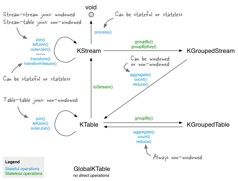
Stateful transformations in the DSL.
We will discuss the various stateful transformations in detail in the subsequent sections. However, let’s start with a first example of a stateful application: the canonical WordCount algorithm.
WordCount example in Java 8+, using lambda expressions (see WordCountLambdaIntegrationTest for the full code):
// We assume record values represent lines of text.  For the sake of this example, we ignore
// whatever may be stored in the record keys.
KStream<String, String> textLines = ...;

KStream<String, Long> wordCounts = textLines
    // Split each text line, by whitespace, into words.  The text lines are the record
    // values, i.e. we can ignore whatever data is in the record keys and thus invoke
    // `flatMapValues` instead of the more generic `flatMap`.
    .flatMapValues(value -> Arrays.asList(value.toLowerCase().split("\\W+")))
    // Group the stream by word to ensure the key of the record is the word.
    .groupBy((key, word) -> word)
    // Count the occurrences of each word (record key).
    //
    // This will change the stream type from `KGroupedStream<String, String>` to
    // `KTable<String, Long>` (word -> count).  We must provide a name for
    // the resulting KTable, which will be used to name e.g. its associated
    // state store and changelog topic.
    .count("Counts")
    // Convert the `KTable<String, Long>` into a `KStream<String, Long>`.
    .toStream();
WordCount example in Java 7:
// Code below is equivalent to the previous Java 8+ example above.
KStream<String, String> textLines = ...;

KStream<String, Long> wordCounts = textLines
    .flatMapValues(new ValueMapper<String, Iterable<String>>() {
        @Override
        public Iterable<String> apply(String value) {
            return Arrays.asList(value.toLowerCase().split("\\W+"));
        }
    })
    .groupBy(new KeyValueMapper<String, String, String>>() {
        @Override
        public String apply(String key, String word) {
            return word;
        }
    })
    .count("Counts")
    .toStream();
Aggregating
Once records are grouped by key via groupByKey or
groupBy – and thus represented as either a KGroupedStream or a KGroupedTable – they can be aggregated
via an operation such as reduce. Aggregations are key-based operations, i.e. they always operate over records
(notably record values) of the same key.
You may choose to perform aggregations on windowed or non-windowed data.
| Transformation | Description |
|---|---|
Aggregate
|
Rolling aggregation. Aggregates the values of (non-windowed) records by the grouped key.
Aggregating is a generalization of When aggregating a grouped stream, you must provide an initializer (think: Several variants of KGroupedStream<byte[], String> groupedStream = ...;
KGroupedTable<byte[], String> groupedTable = ...;
// Java 8+ examples, using lambda expressions
// Aggregating a KGroupedStream (note how the value type changes from String to Long)
KTable<byte[], Long> aggregatedStream = groupedStream.aggregate(
() -> 0L, /* initializer */
(aggKey, newValue, aggValue) -> aggValue + newValue.length(), /* adder */
Serdes.Long(), /* serde for aggregate value */
"aggregated-stream-store" /* state store name */);
// Aggregating a KGroupedTable (note how the value type changes from String to Long)
KTable<byte[], Long> aggregatedTable = groupedTable.aggregate(
() -> 0L, /* initializer */
(aggKey, newValue, aggValue) -> aggValue + newValue.length(), /* adder */
(aggKey, oldValue, aggValue) -> aggValue - oldValue.length(), /* subtractor */
Serdes.Long(), /* serde for aggregate value */
"aggregated-table-store" /* state store name */);
// Java 7 examples
// Aggregating a KGroupedStream (note how the value type changes from String to Long)
KTable<byte[], Long> aggregatedStream = groupedStream.aggregate(
new Initializer<Long>() { /* initializer */
@Override
public Long apply() {
return 0L;
}
},
new Aggregator<byte[], String, Long>() { /* adder */
@Override
public Long apply(byte[] aggKey, String newValue, Long aggValue) {
return aggValue + newValue.length();
}
},
Serdes.Long(),
"aggregated-stream-store");
// Aggregating a KGroupedTable (note how the value type changes from String to Long)
KTable<byte[], Long> aggregatedTable = groupedTable.aggregate(
new Initializer<Long>() { /* initializer */
@Override
public Long apply() {
return 0L;
}
},
new Aggregator<byte[], String, Long>() { /* adder */
@Override
public Long apply(byte[] aggKey, String newValue, Long aggValue) {
return aggValue + newValue.length();
}
},
new Aggregator<byte[], String, Long>() { /* subtractor */
@Override
public Long apply(byte[] aggKey, String oldValue, Long aggValue) {
return aggValue - oldValue.length();
}
},
Serdes.Long(),
"aggregated-table-store");
Detailed behavior of
Detailed behavior of
See the example at the bottom of this section for a visualization of the aggregation semantics. |
Aggregate (windowed)
|
Windowed aggregation.
Aggregates the values of records, per window, by the grouped key.
Aggregating is a generalization of You must provide an initializer (think: The windowed Several variants of import java.util.concurrent.TimeUnit;
KGroupedStream<String, Long> groupedStream = ...;
// Java 8+ examples, using lambda expressions
// Aggregating with time-based windowing (here: with 5-minute tumbling windows)
KTable<Windowed<String>, Long> timeWindowedAggregatedStream = groupedStream.aggregate(
() -> 0L, /* initializer */
(aggKey, newValue, aggValue) -> aggValue + newValue, /* adder */
TimeWindows.of(TimeUnit.MINUTES.toMillis(5)), /* time-based window */
Serdes.Long(), /* serde for aggregate value */
"time-windowed-aggregated-stream-store" /* state store name */);
// Aggregating with session-based windowing (here: with an inactivity gap of 5 minutes)
KTable<Windowed<String>, Long> sessionizedAggregatedStream = groupedStream.aggregate(
() -> 0L, /* initializer */
(aggKey, newValue, aggValue) -> aggValue + newValue, /* adder */
(aggKey, leftAggValue, rightAggValue) -> leftAggValue + rightAggValue, /* session merger */
SessionWindows.with(TimeUnit.MINUTES.toMillis(5)), /* session window */
Serdes.Long(), /* serde for aggregate value */
"sessionized-aggregated-stream-store" /* state store name */);
// Java 7 examples
// Aggregating with time-based windowing (here: with 5-minute tumbling windows)
KTable<Windowed<String>, Long> timeWindowedAggregatedStream = groupedStream.aggregate(
new Initializer<Long>() { /* initializer */
@Override
public Long apply() {
return 0L;
}
},
new Aggregator<String, Long, Long>() { /* adder */
@Override
public Long apply(String aggKey, Long newValue, Long aggValue) {
return aggValue + newValue;
}
},
TimeWindows.of(TimeUnit.MINUTES.toMillis(5)), /* time-based window */
Serdes.Long(), /* serde for aggregate value */
"time-windowed-aggregated-stream-store" /* state store name */);
// Aggregating with session-based windowing (here: with an inactivity gap of 5 minutes)
KTable<Windowed<String>, Long> sessionizedAggregatedStream = groupedStream.aggregate(
new Initializer<Long>() { /* initializer */
@Override
public Long apply() {
return 0L;
}
},
new Aggregator<String, Long, Long>() { /* adder */
@Override
public Long apply(String aggKey, Long newValue, Long aggValue) {
return aggValue + newValue;
}
},
new Merger<String, Long>() { /* session merger */
@Override
public Long apply(String aggKey, Long leftAggValue, Long rightAggValue) {
return rightAggValue + leftAggValue;
}
},
SessionWindows.with(TimeUnit.MINUTES.toMillis(5)), /* session window */
Serdes.Long(), /* serde for aggregate value */
"sessionized-aggregated-stream-store" /* state store name */);
Detailed behavior:
See the example at the bottom of this section for a visualization of the aggregation semantics. |
Count
|
Rolling aggregation. Counts the number of records by the grouped key. (KGroupedStream details, KGroupedTable details) Several variants of KGroupedStream<String, Long> groupedStream = ...;
KGroupedTable<String, Long> groupedTable = ...;
// Counting a KGroupedStream
KTable<String, Long> aggregatedStream = groupedStream.count(
"counted-stream-store" /* state store name */);
// Counting a KGroupedTable
KTable<String, Long> aggregatedTable = groupedTable.count(
"counted-table-store" /* state store name */);
Detailed behavior for
Detailed behavior for
|
Count (windowed)
|
Windowed aggregation. Counts the number of records, per window, by the grouped key. (KGroupedStream details) The windowed Several variants of import java.util.concurrent.TimeUnit;
KGroupedStream<String, Long> groupedStream = ...;
// Counting a KGroupedStream with time-based windowing (here: with 5-minute tumbling windows)
KTable<Windowed<String>, Long> aggregatedStream = groupedStream.count(
TimeWindows.of(TimeUnit.MINUTES.toMillis(5)), /* time-based window */
"time-windowed-counted-stream-store" /* state store name */);
// Counting a KGroupedStream with session-based windowing (here: with 5-minute inactivity gaps)
KTable<Windowed<String>, Long> aggregatedStream = groupedStream.count(
SessionWindows.with(TimeUnit.MINUTES.toMillis(5)), /* session window */
"sessionized-counted-stream-store" /* state store name */);
Detailed behavior:
|
Reduce
|
Rolling aggregation. Combines the values of (non-windowed) records by the grouped key.
The current record value is combined with the last reduced value, and a new reduced value is returned.
The result value type cannot be changed, unlike When reducing a grouped stream, you must provide an “adder” reducer (think: Several variants of KGroupedStream<String, Long> groupedStream = ...;
KGroupedTable<String, Long> groupedTable = ...;
// Java 8+ examples, using lambda expressions
// Reducing a KGroupedStream
KTable<String, Long> aggregatedStream = groupedStream.reduce(
(aggValue, newValue) -> aggValue + newValue, /* adder */
"reduced-stream-store" /* state store name */);
// Reducing a KGroupedTable
KTable<String, Long> aggregatedTable = groupedTable.reduce(
(aggValue, newValue) -> aggValue + newValue, /* adder */
(aggValue, oldValue) -> aggValue - oldValue, /* subtractor */
"reduced-table-store" /* state store name */);
// Java 7 examples
// Reducing a KGroupedStream
KTable<String, Long> aggregatedStream = groupedStream.reduce(
new Reducer<Long>() { /* adder */
@Override
public Long apply(Long aggValue, Long newValue) {
return aggValue + newValue;
}
},
"reduced-stream-store" /* state store name */);
// Reducing a KGroupedTable
KTable<String, Long> aggregatedTable = groupedTable.reduce(
new Reducer<Long>() { /* adder */
@Override
public Long apply(Long aggValue, Long newValue) {
return aggValue + newValue;
}
},
new Reducer<Long>() { /* subtractor */
@Override
public Long apply(Long aggValue, Long oldValue) {
return aggValue - oldValue;
}
},
"reduced-table-store" /* state store name */);
Detailed behavior for
Detailed behavior for
See the example at the bottom of this section for a visualization of the aggregation semantics. |
Reduce (windowed)
|
Windowed aggregation.
Combines the values of records, per window, by the grouped key.
The current record value is combined with the last reduced value, and a new reduced value is returned.
Records with The windowed Several variants of import java.util.concurrent.TimeUnit;
KGroupedStream<String, Long> groupedStream = ...;
// Java 8+ examples, using lambda expressions
// Aggregating with time-based windowing (here: with 5-minute tumbling windows)
KTable<Windowed<String>, Long> timeWindowedAggregatedStream = groupedStream.reduce(
(aggValue, newValue) -> aggValue + newValue, /* adder */
TimeWindows.of(TimeUnit.MINUTES.toMillis(5)), /* time-based window */
"time-windowed-reduced-stream-store" /* state store name */);
// Aggregating with session-based windowing (here: with an inactivity gap of 5 minutes)
KTable<Windowed<String>, Long> sessionzedAggregatedStream = groupedStream.reduce(
(aggValue, newValue) -> aggValue + newValue, /* adder */
SessionWindows.with(TimeUnit.MINUTES.toMillis(5)), /* session window */
"sessionized-reduced-stream-store" /* state store name */);
// Java 7 examples
// Aggregating with time-based windowing (here: with 5-minute tumbling windows)
KTable<Windowed<String>, Long> timeWindowedAggregatedStream = groupedStream.reduce(
new Reducer<Long>() { /* adder */
@Override
public Long apply(Long aggValue, Long newValue) {
return aggValue + newValue;
}
},
TimeWindows.of(TimeUnit.MINUTES.toMillis(5)), /* time-based window */
"time-windowed-reduced-stream-store" /* state store name */);
// Aggregating with session-based windowing (here: with an inactivity gap of 5 minutes)
KTable<Windowed<String>, Long> timeWindowedAggregatedStream = groupedStream.reduce(
new Reducer<Long>() { /* adder */
@Override
public Long apply(Long aggValue, Long newValue) {
return aggValue + newValue;
}
},
SessionWindows.with(TimeUnit.MINUTES.toMillis(5)), /* session window */
"sessionized-reduced-stream-store" /* state store name */);
Detailed behavior:
See the example at the bottom of this section for a visualization of the aggregation semantics. |
Example of semantics for stream aggregations:
A KGroupedStream → KTable example is shown below. The streams and the table are initially empty. We use bold
font in the column for “KTable aggregated” to highlight changed state. An entry such as (hello, 1) denotes a
record with key hello and value 1. To improve the readability of the semantics table we assume that all records
are processed in timestamp order.
// Key: word, value: count
KStream<String, Integer> wordCounts = ...;

KGroupedStream<String, Integer> groupedStream = wordCounts
    .groupByKey(Serdes.String(), Serdes.Integer());

KTable<String, Integer> aggregated = groupedStream.aggregate(
    () -> 0, /* initializer */
    (aggKey, newValue, aggValue) -> aggValue + newValue, /* adder */
    Serdes.Integer(), /* serde for aggregate value */
    "aggregated-stream-store" /* state store name */);
Note
Impact of record caches:
For illustration purposes, the column “KTable aggregated” below shows the table’s state changes over time in a
very granular way. In practice, you would observe state changes in such a granular way only when
record caches are disabled (default: enabled).
When record caches are enabled, what might happen for example is that the output results of the rows with timestamps
4 and 5 would be compacted, and there would only be
a single state update for the key kafka in the KTable (here: from (kafka 1) directly to (kafka, 3).
Typically, you should only disable record caches for testing or debugging purposes – under normal circumstances it
is better to leave record caches enabled.
KStream wordCounts |
KGroupedStream groupedStream |
KTable aggregated |
|||
|---|---|---|---|---|---|
| Timestamp | Input record | Grouping | Initializer | Adder | State |
| 1 | (hello, 1) | (hello, 1) | 0 (for hello) | (hello, 0 + 1) | (hello, 1)
|
| 2 | (kafka, 1) | (kafka, 1) | 0 (for kafka) | (kafka, 0 + 1) | (hello, 1)
(kafka, 1)
|
| 3 | (streams, 1) | (streams, 1) | 0 (for streams) | (streams, 0 + 1) | (hello, 1)
(kafka, 1)
(streams, 1)
|
| 4 | (kafka, 1) | (kafka, 1) | (kafka, 1 + 1) | (hello, 1)
(kafka, 2)
(streams, 1)
|
|
| 5 | (kafka, 1) | (kafka, 1) | (kafka, 2 + 1) | (hello, 1)
(kafka, 3)
(streams, 1)
|
|
| 6 | (streams, 1) | (streams, 1) | (streams, 1 + 1) | (hello, 1)
(kafka, 3)
(streams, 2)
|
|
Example of semantics for table aggregations:
A KGroupedTable → KTable example is shown below. The tables are initially empty. We use bold font in the column
for “KTable aggregated” to highlight changed state. An entry such as (hello, 1) denotes a record with key
hello and value 1. To improve the readability of the semantics table we assume that all records are processed
in timestamp order.
// Key: username, value: user region (abbreviated to "E" for "Europe", "A" for "Asia")
KTable<String, String> userProfiles = ...;

// Re-group `userProfiles`.  Don't read too much into what the grouping does:
// its prime purpose in this example is to show the *effects* of the grouping
// in the subsequent aggregation.
KGroupedTable<String, Integer> groupedTable = userProfiles
    .groupBy((user, region) -> KeyValue.pair(region, user.length()), Serdes.String(), Serdes.Integer());

KTable<String, Integer> aggregated = groupedTable.aggregate(
    () -> 0, /* initializer */
    (aggKey, newValue, aggValue) -> aggValue + newValue, /* adder */
    (aggKey, oldValue, aggValue) -> aggValue - oldValue, /* subtractor */
    Serdes.Integer(), /* serde for aggregate value */
    "aggregated-table-store" /* state store name */);
Note
Impact of record caches:
For illustration purposes, the column “KTable aggregated” below shows the table’s state changes over time in a
very granular way. In practice, you would observe state changes in such a granular way only when
record caches are disabled (default: enabled).
When record caches are enabled, what might happen for example is that the output results of the rows with timestamps
4 and 5 would be compacted, and there would only be
a single state update for the key kafka in the KTable (here: from (kafka 1) directly to (kafka, 3).
Typically, you should only disable record caches for testing or debugging purposes – under normal circumstances it
is better to leave record caches enabled.
KTable userProfiles |
KGroupedTable groupedTable |
KTable aggregated |
|||||
|---|---|---|---|---|---|---|---|
| Timestamp | Input record | Interpreted as | Grouping | Initializer | Adder | Subtractor | State |
| 1 | (alice, E) | INSERT alice | (E, 5) | 0 (for E) | (E, 0 + 5) | (E, 5)
|
|
| 2 | (bob, A) | INSERT bob | (A, 3) | 0 (for A) | (A, 0 + 3) | (A, 3)
(E, 5)
|
|
| 3 | (charlie, A) | INSERT charlie | (A, 7) | (A, 3 + 7) | (A, 10)
(E, 5)
|
||
| 4 | (alice, A) | UPDATE alice | (A, 5) | (A, 10 + 5) | (E, 5 - 5) | (A, 15)
(E, 0)
|
|
| 5 | (charlie, null) | DELETE charlie | (null, 7) | (A, 15 - 7) | (A, 8)
(E, 0)
|
||
| 6 | (null, E) | ignored | (A, 8)
(E, 0)
|
||||
| 7 | (bob, E) | UPDATE bob | (E, 3) | (E, 0 + 3) | (A, 8 - 3) | (A, 5)
(E, 3)
|
|
Joining
Streams and tables can also be joined. Many stream processing applications in practice are coded as streaming joins. For example, applications backing an online shop might need to access multiple, updating database tables (e.g. sales prices, inventory, customer information) in order to enrich a new data record (e.g. customer transaction) with context information. That is, scenarios where you need to perform table lookups at very large scale and with a low processing latency. Here, a popular pattern is to make the information in the databases available in Kafka through so-called change data capture in combination with Kafka’s Connect API, and then implementing applications that leverage the Streams API to perform very fast and efficient local joins of such tables and streams, rather than requiring the application to make a query to a remote database over the network for each record. In this example, the KTable concept in Kafka Streams would enable you to track the latest state (think: snapshot) of each table in a local state store, thus greatly reducing the processing latency as well as reducing the load of the remote databases when doing such streaming joins.
The following join operations are supported, see also the diagram in the overview section of Stateful Transformations. Depending on the operands, joins are either windowed joins or non-windowed joins.
| Join operands | Type | (INNER) JOIN | LEFT JOIN | OUTER JOIN | Demo application |
|---|---|---|---|---|---|
| KStream-to-KStream | Windowed | Supported | Supported | Supported | StreamToStreamJoinIntegrationTest |
| KTable-to-KTable | Non-windowed | Supported | Supported | Supported | TableToTableJoinIntegrationTest |
| KStream-to-KTable | Non-windowed | Supported | Supported | Not Supported | StreamToTableJoinIntegrationTest |
| KStream-to-GlobalKTable | Non-windowed | Supported | Supported | Not Supported | GlobalKTablesExample |
| KTable-to-GlobalKTable | N/A | Not Supported | Not Supported | Not Supported | N/A |
We explain each case in more detail in the subsequent sections.
Input data must be co-partitioned as described below when joining to ensure that input records with the same key (from both sides of the join) are delivered to the same stream task during processing. It is the responsibility of the user to ensure data co-partitioning when joining.
Tip
If your use case allows for it, you should consider using global tables aka
GlobalKTable for joining because, among other reasons, they do not require data co-partitioning.
The requirements for data co-partitioning are:
- The input topics of the join (left side and right side) must have the same number of partitions.
- All applications that write to the input topics must have the same partitioning strategy so that records with
the same key are delivered to same partition number. In other words, the keyspace of the input data must be
distributed across partitions in the same manner.
This means that, for example, applications that use Kafka’s Java Producer API must use the
same partitioner (cf. the producer setting
"partitioner.class"akaProducerConfig.PARTITIONER_CLASS_CONFIG), and applications that use the Kafka’s Streams API must use the sameStreamPartitionerfor operations such asKStream#to(). The good news is that, if you happen to use the default partitioner-related settings across all applications, you do not need to worry about the partitioning strategy.
Why is data co-partitioning required? Because
KStream-KStream,
KTable-KTable, and
KStream-KTable joins
are performed based on the keys of records (think: leftRecord.key == rightRecord.key), it is required that the
input streams/tables of a join are co-partitioned by key.
The only exception are
KStream-GlobalKTable joins. Here, co-partitioning is
it not required because all partitions of the GlobalKTable‘s underlying changelog stream are made available to
each KafkaStreams instance, i.e. each instance has a full copy of the changelog stream. Further, a
KeyValueMapper allows for non-key based joins from the KStream to the GlobalKTable.
Note
Kafka Streams partly verifies the co-partitioning requirement:
During the partition assignment step, i.e. at runtime, Kafka Streams verifies whether the number of partitions for
both sides of a join are the same. If they are not, a TopologyBuilderException (runtime exception) is being
thrown. Note that Kafka Streams cannot verify whether the partitioning strategy matches between the input
streams/tables of a join – it is up to the user to ensure that this is the case.
Ensuring data co-partitioning: If the inputs of a join are not co-partitioned yet, you must ensure this manually. You may follow a procedure such as outlined below.
Identify the input KStream/KTable in the join whose underlying Kafka topic has the smaller number of partitions. Let’s call this stream/table “SMALLER”, and the other side of the join “LARGER”. To learn about the number of partitions of a Kafka topic you can use, for example, the CLI tool
bin/kafka-topicswith the--describeoption.Pre-create a new Kafka topic for “SMALLER” that has the same number of partitions as “LARGER”. Let’s call this new topic “repartitioned-topic-for-smaller”. Typically, you’d use the CLI tool
bin/kafka-topicswith the--createoption for this.Within your application, re-write the data of “SMALLER” into the new Kafka topic. You must ensure that, when writing the data with
toorthrough, the same partitioner is used as for “LARGER”.- If “SMALLER” is a KStream:
KStream#to("repartitioned-topic-for-smaller"). - If “SMALLER” is a KTable:
KTable#to("repartitioned-topic-for-smaller").
- If “SMALLER” is a KStream:
Within your application, re-read the data in “repartitioned-topic-for-smaller” into a new KStream/KTable.
- If “SMALLER” is a KStream:
KStreamBuilder#stream("repartitioned-topic-for-smaller"). - If “SMALLER” is a KTable:
KStreamBuilder#table("repartitioned-topic-for-smaller").
- If “SMALLER” is a KStream:
Within your application, perform the join between “LARGER” and the new stream/table.
KStream-KStream joins are always windowed joins, because otherwise the size of the internal state store used to perform the join – think: a sliding window or “buffer” – would grow indefinitely. For stream-stream joins it’s important to highlight that a new input record on one side will produce a join output for each matching record on the other side, and there can be multiple such matching records in a given join window (cf. the row with timestamp 15 in the join semantics table below, for example).
Join output records are effectively created as follows, leveraging the user-supplied ValueJoiner:
KeyValue<K, LV> leftRecord = ...;
KeyValue<K, RV> rightRecord = ...;
ValueJoiner<LV, RV, JV> joiner = ...;

KeyValue<K, JV> joinOutputRecord = KeyValue.pair(
    leftRecord.key, /* by definition, leftRecord.key == rightRecord.key */
    joiner.apply(leftRecord.value, rightRecord.value)
  );
| Transformation | Description |
|---|---|
Inner Join (windowed)
|
Performs an INNER JOIN of this stream with another stream.
Even though this operation is windowed, the joined stream will be of type Data must be co-partitioned: The input data for both sides must be co-partitioned. Causes data re-partitioning of a stream if and only if the stream was marked for re-partitioning (if both are marked, both are re-partitioned). Several variants of import java.util.concurrent.TimeUnit;
KStream<String, Long> left = ...;
KStream<String, Double> right = ...;
// Java 8+ example, using lambda expressions
KStream<String, String> joined = left.join(right,
(leftValue, rightValue) -> "left=" + leftValue + ", right=" + rightValue, /* ValueJoiner */
JoinWindows.of(TimeUnit.MINUTES.toMillis(5)),
Serdes.String(), /* key */
Serdes.Long(), /* left value */
Serdes.Double() /* right value */
);
// Java 7 example
KStream<String, String> joined = left.join(right,
new ValueJoiner<Long, Double, String>() {
@Override
public String apply(Long leftValue, Double rightValue) {
return "left=" + leftValue + ", right=" + rightValue;
}
},
JoinWindows.of(TimeUnit.MINUTES.toMillis(5)),
Serdes.String(), /* key */
Serdes.Long(), /* left value */
Serdes.Double() /* right value */
);
Detailed behavior:
See the semantics overview at the bottom of this section for a detailed description. |
Left Join (windowed)
|
Performs a LEFT JOIN of this stream with another stream.
Even though this operation is windowed, the joined stream will be of type Data must be co-partitioned: The input data for both sides must be co-partitioned. Causes data re-partitioning of a stream if and only if the stream was marked for re-partitioning (if both are marked, both are re-partitioned). Several variants of import java.util.concurrent.TimeUnit;
KStream<String, Long> left = ...;
KStream<String, Double> right = ...;
// Java 8+ example, using lambda expressions
KStream<String, String> joined = left.leftJoin(right,
(leftValue, rightValue) -> "left=" + leftValue + ", right=" + rightValue, /* ValueJoiner */
JoinWindows.of(TimeUnit.MINUTES.toMillis(5)),
Serdes.String(), /* key */
Serdes.Long(), /* left value */
Serdes.Double() /* right value */
);
// Java 7 example
KStream<String, String> joined = left.leftJoin(right,
new ValueJoiner<Long, Double, String>() {
@Override
public String apply(Long leftValue, Double rightValue) {
return "left=" + leftValue + ", right=" + rightValue;
}
},
JoinWindows.of(TimeUnit.MINUTES.toMillis(5)),
Serdes.String(), /* key */
Serdes.Long(), /* left value */
Serdes.Double() /* right value */
);
Detailed behavior:
See the semantics overview at the bottom of this section for a detailed description. |
Outer Join (windowed)
|
Performs an OUTER JOIN of this stream with another stream.
Even though this operation is windowed, the joined stream will be of type Data must be co-partitioned: The input data for both sides must be co-partitioned. Causes data re-partitioning of a stream if and only if the stream was marked for re-partitioning (if both are marked, both are re-partitioned). Several variants of import java.util.concurrent.TimeUnit;
KStream<String, Long> left = ...;
KStream<String, Double> right = ...;
// Java 8+ example, using lambda expressions
KStream<String, String> joined = left.outerJoin(right,
(leftValue, rightValue) -> "left=" + leftValue + ", right=" + rightValue, /* ValueJoiner */
JoinWindows.of(TimeUnit.MINUTES.toMillis(5)),
Serdes.String(), /* key */
Serdes.Long(), /* left value */
Serdes.Double() /* right value */
);
// Java 7 example
KStream<String, String> joined = left.outerJoin(right,
new ValueJoiner<Long, Double, String>() {
@Override
public String apply(Long leftValue, Double rightValue) {
return "left=" + leftValue + ", right=" + rightValue;
}
},
JoinWindows.of(TimeUnit.MINUTES.toMillis(5)),
Serdes.String(), /* key */
Serdes.Long(), /* left value */
Serdes.Double() /* right value */
);
Detailed behavior:
See the semantics overview at the bottom of this section for a detailed description. |
Semantics of stream-stream joins:
The semantics of the various stream-stream join variants are explained below.
To improve the readability of the table we assume that (1) all records have the same key (and thus we omit the key in
the table), (2) all records belong to a single join window, and (3) all records are processed in timestamp order.
The columns INNER JOIN, LEFT JOIN, and OUTER JOIN denote what is passed as arguments to the user-supplied
ValueJoiner for the join, leftJoin, and
outerJoin methods, respectively, whenever a new input record is received on either side of the join. An empty table
cell denotes that the ValueJoiner is not called at all.
| Timestamp | Left (KStream) | Right (KStream) | (INNER) JOIN | LEFT JOIN | OUTER JOIN |
|---|---|---|---|---|---|
| 1 | null | ||||
| 2 | null | ||||
| 3 | A | [A, null] | [A, null] | ||
| 4 | a | [A, a] | [A, a] | [A, a] | |
| 5 | B | [B, a] | [B, a] | [B, a] | |
| 6 | b | [A, b], [B, b] | [A, b], [B, b] | [A, b], [B, b] | |
| 7 | null | ||||
| 8 | null | ||||
| 9 | C | [C, a], [C, b] | [C, a], [C, b] | [C, a], [C, b] | |
| 10 | c | [A, c], [B, c], [C, c] | [A, c], [B, c], [C, c] | [A, c], [B, c], [C, c] | |
| 11 | null | ||||
| 12 | null | ||||
| 13 | null | ||||
| 14 | d | [A, d], [B, d], [C, d] | [A, d], [B, d], [C, d] | [A, d], [B, d], [C, d] | |
| 15 | D | [D, a], [D, b], [D, c], [D, d] | [D, a], [D, b], [D, c], [D, d] | [D, a], [D, b], [D, c], [D, d] |
KTable-KTable joins are always non-windowed joins. They are designed to be consistent with their counterparts in relational databases. The changelog streams of both KTables are materialized into local state stores to represent the latest snapshot of their table duals. The join result is a new KTable that represents the changelog stream of the join operation.
Join output records are effectively created as follows, leveraging the user-supplied ValueJoiner:
KeyValue<K, LV> leftRecord = ...;
KeyValue<K, RV> rightRecord = ...;
ValueJoiner<LV, RV, JV> joiner = ...;

KeyValue<K, JV> joinOutputRecord = KeyValue.pair(
    leftRecord.key, /* by definition, leftRecord.key == rightRecord.key */
    joiner.apply(leftRecord.value, rightRecord.value)
  );
| Transformation | Description |
|---|---|
Inner Join
|
Performs an INNER JOIN of this table with another table. The result is an ever-updating KTable that represents the “current” result of the join. (details) Data must be co-partitioned: The input data for both sides must be co-partitioned. KTable<String, Long> left = ...;
KTable<String, Double> right = ...;
// Java 8+ example, using lambda expressions
KTable<String, String> joined = left.join(right,
(leftValue, rightValue) -> "left=" + leftValue + ", right=" + rightValue /* ValueJoiner */
);
// Java 7 example
KTable<String, String> joined = left.join(right,
new ValueJoiner<Long, Double, String>() {
@Override
public String apply(Long leftValue, Double rightValue) {
return "left=" + leftValue + ", right=" + rightValue;
}
});
Detailed behavior:
See the semantics overview at the bottom of this section for a detailed description. |
Left Join
|
Performs a LEFT JOIN of this table with another table. (details) Data must be co-partitioned: The input data for both sides must be co-partitioned. KTable<String, Long> left = ...;
KTable<String, Double> right = ...;
// Java 8+ example, using lambda expressions
KTable<String, String> joined = left.leftJoin(right,
(leftValue, rightValue) -> "left=" + leftValue + ", right=" + rightValue /* ValueJoiner */
);
// Java 7 example
KTable<String, String> joined = left.leftJoin(right,
new ValueJoiner<Long, Double, String>() {
@Override
public String apply(Long leftValue, Double rightValue) {
return "left=" + leftValue + ", right=" + rightValue;
}
});
Detailed behavior:
See the semantics overview at the bottom of this section for a detailed description. |
Outer Join
|
Performs an OUTER JOIN of this table with another table. (details) Data must be co-partitioned: The input data for both sides must be co-partitioned. KTable<String, Long> left = ...;
KTable<String, Double> right = ...;
// Java 8+ example, using lambda expressions
KTable<String, String> joined = left.outerJoin(right,
(leftValue, rightValue) -> "left=" + leftValue + ", right=" + rightValue /* ValueJoiner */
);
// Java 7 example
KTable<String, String> joined = left.outerJoin(right,
new ValueJoiner<Long, Double, String>() {
@Override
public String apply(Long leftValue, Double rightValue) {
return "left=" + leftValue + ", right=" + rightValue;
}
});
Detailed behavior:
See the semantics overview at the bottom of this section for a detailed description. |
Semantics of table-table joins:
The semantics of the various table-table join variants are explained below.
To improve the readability of the table we assume that (1) all records have the same key (and thus we omit the key in
the table) and that (2) all records are processed in timestamp order.
The columns INNER JOIN, LEFT JOIN, and OUTER JOIN denote what is passed as arguments to the user-supplied
ValueJoiner for the join, leftJoin, and
outerJoin methods, respectively, whenever a new input record is received on either side of the join. An empty table
cell denotes that the ValueJoiner is not called at all.
| Timestamp | Left (KTable) | Right (KTable) | (INNER) JOIN | LEFT JOIN | OUTER JOIN |
|---|---|---|---|---|---|
| 1 | null (tombstone) | ||||
| 2 | null (tombstone) | ||||
| 3 | A | [A, null] | [A, null] | ||
| 4 | a | [A, a] | [A, a] | [A, a] | |
| 5 | B | [B, a] | [B, a] | [B, a] | |
| 6 | b | [B, b] | [B, b] | [B, b] | |
| 7 | null (tombstone) | null (tombstone) | null (tombstone) | [null, b] | |
| 8 | null (tombstone) | null (tombstone) | |||
| 9 | C | [C, null] | [C, null] | ||
| 10 | c | [C, c] | [C, c] | [C, c] | |
| 11 | null (tombstone) | null (tombstone) | [C, null] | [C, null] | |
| 12 | null (tombstone) | null (tombstone) | null (tombstone) | ||
| 13 | null (tombstone) | ||||
| 14 | d | [null, d] | |||
| 15 | D | [D, d] | [D, d] | [D, d] |
KStream-KTable joins are always non-windowed joins. They allow you to perform table lookups against a KTable (changelog stream) upon receiving a new record from the KStream (record stream). An example use case would be to enrich a stream of user activities (KStream) with the latest user profile information (KTable).
Join output records are effectively created as follows, leveraging the user-supplied ValueJoiner:
KeyValue<K, LV> leftRecord = ...;
KeyValue<K, RV> rightRecord = ...;
ValueJoiner<LV, RV, JV> joiner = ...;

KeyValue<K, JV> joinOutputRecord = KeyValue.pair(
    leftRecord.key, /* by definition, leftRecord.key == rightRecord.key */
    joiner.apply(leftRecord.value, rightRecord.value)
  );
| Transformation | Description |
|---|---|
Inner Join
|
Performs an INNER JOIN of this stream with the table, effectively doing a table lookup. (details) Data must be co-partitioned: The input data for both sides must be co-partitioned. Causes data re-partitioning of the stream if and only if the stream was marked for re-partitioning. Several variants of KStream<String, Long> left = ...;
KTable<String, Double> right = ...;
// Java 8+ example, using lambda expressions
KStream<String, String> joined = left.join(right,
(leftValue, rightValue) -> "left=" + leftValue + ", right=" + rightValue, /* ValueJoiner */
Serdes.String(), /* key */
Serdes.Long() /* left value */
);
// Java 7 example
KStream<String, String> joined = left.join(right,
new ValueJoiner<Long, Double, String>() {
@Override
public String apply(Long leftValue, Double rightValue) {
return "left=" + leftValue + ", right=" + rightValue;
}
},
Serdes.String(), /* key */
Serdes.Long() /* left value */
);
Detailed behavior:
See the semantics overview at the bottom of this section for a detailed description. |
Left Join
|
Performs a LEFT JOIN of this stream with the table, effectively doing a table lookup. (details) Data must be co-partitioned: The input data for both sides must be co-partitioned. Causes data re-partitioning of the stream if and only if the stream was marked for re-partitioning. Several variants of KStream<String, Long> left = ...;
KTable<String, Double> right = ...;
// Java 8+ example, using lambda expressions
KStream<String, String> joined = left.leftJoin(right,
(leftValue, rightValue) -> "left=" + leftValue + ", right=" + rightValue, /* ValueJoiner */
Serdes.String(), /* key */
Serdes.Long() /* left value */
);
// Java 7 example
KStream<String, String> joined = left.leftJoin(right,
new ValueJoiner<Long, Double, String>() {
@Override
public String apply(Long leftValue, Double rightValue) {
return "left=" + leftValue + ", right=" + rightValue;
}
},
Serdes.String(), /* key */
Serdes.Long() /* left value */
);
Detailed behavior:
See the semantics overview at the bottom of this section for a detailed description. |
Semantics of stream-table joins:
The semantics of the various stream-table join variants are explained below.
To improve the readability of the table we assume that (1) all records have the same key (and thus we omit the key in
the table) and that (2) all records are processed in timestamp order.
The columns INNER JOIN and LEFT JOIN denote what is passed as arguments to the user-supplied
ValueJoiner for the join and leftJoin
methods, respectively, whenever a new input record is received on either side of the join. An empty table
cell denotes that the ValueJoiner is not called at all.
| Timestamp | Left (KStream) | Right (KTable) | (INNER) JOIN | LEFT JOIN |
|---|---|---|---|---|
| 1 | null | |||
| 2 | null (tombstone) | |||
| 3 | A | [A, null] | ||
| 4 | a | |||
| 5 | B | [B, a] | [B, a] | |
| 6 | b | |||
| 7 | null | |||
| 8 | null (tombstone) | |||
| 9 | C | [C, null] | ||
| 10 | c | |||
| 11 | null | |||
| 12 | null | |||
| 13 | null | |||
| 14 | d | |||
| 15 | D | [D, d] | [D, d] |
KStream-GlobalKTable joins are always non-windowed joins. They allow you to perform table lookups against a GlobalKTable (entire changelog stream) upon receiving a new record from the KStream (record stream). An example use case would be “star queries” or “star joins”, where you would enrich a stream of user activities (KStream) with the latest user profile information (GlobalKTable) and further context information (further GlobalKTables).
At a high-level, KStream-GlobalKTable joins are very similar to KStream-KTable joins. However, global tables provide you with much more flexibility at the some expense when compared to partitioned tables:
- They do not require data co-partitioning.
- They allow for efficient “star joins”; i.e., joining a large-scale “facts” stream against “dimension” tables
- They allow for joining against foreign keys; i.e., you can lookup data in the table not just by the keys of records in the stream, but also by data in the record values.
- They make many use cases feasible where you must work on heavily skewed data and thus suffer from hot partitions.
- They are often more efficient than their partitioned KTable counterpart when you need to perform multiple joins in succession.
Join output records are effectively created as follows, leveraging the user-supplied ValueJoiner:
KeyValue<K, LV> leftRecord = ...;
KeyValue<K, RV> rightRecord = ...;
ValueJoiner<LV, RV, JV> joiner = ...;

KeyValue<K, JV> joinOutputRecord = KeyValue.pair(
    leftRecord.key, /* by definition, leftRecord.key == rightRecord.key */
    joiner.apply(leftRecord.value, rightRecord.value)
  );
| Transformation | Description |
|---|---|
Inner Join
|
Performs an INNER JOIN of this stream with the global table, effectively doing a table lookup. (details) The Causes data re-partitioning of the stream if and only if the stream was marked for re-partitioning. KStream<String, Long> left = ...;
GlobalKTable<Integer, Double> right = ...;
// Java 8+ example, using lambda expressions
KStream<String, String> joined = left.join(right,
(leftKey, leftValue) -> leftKey.length(), /* derive a (potentially) new key by which to lookup against the table */
(leftValue, rightValue) -> "left=" + leftValue + ", right=" + rightValue /* ValueJoiner */
);
// Java 7 example
KStream<String, String> joined = left.join(right,
new KeyValueMapper<String, Long, Integer>() { /* derive a (potentially) new key by which to lookup against the table */
@Override
public Integer apply(String key, Long value) {
return key.length();
}
},
new ValueJoiner<Long, Double, String>() {
@Override
public String apply(Long leftValue, Double rightValue) {
return "left=" + leftValue + ", right=" + rightValue;
}
});
Detailed behavior:
|
Left Join
|
Performs a LEFT JOIN of this stream with the global table, effectively doing a table lookup. (details) The Causes data re-partitioning of the stream if and only if the stream was marked for re-partitioning. KStream<String, Long> left = ...;
GlobalKTable<Integer, Double> right = ...;
// Java 8+ example, using lambda expressions
KStream<String, String> joined = left.leftJoin(right,
(leftKey, leftValue) -> leftKey.length(), /* derive a (potentially) new key by which to lookup against the table */
(leftValue, rightValue) -> "left=" + leftValue + ", right=" + rightValue /* ValueJoiner */
);
// Java 7 example
KStream<String, String> joined = left.leftJoin(right,
new KeyValueMapper<String, Long, Integer>() { /* derive a (potentially) new key by which to lookup against the table */
@Override
public Integer apply(String key, Long value) {
return key.length();
}
},
new ValueJoiner<Long, Double, String>() {
@Override
public String apply(Long leftValue, Double rightValue) {
return "left=" + leftValue + ", right=" + rightValue;
}
});
Detailed behavior:
|
Semantics of stream-table joins:
The join semantics are identical to KStream-KTable joins.
The only difference is that, for KStream-GlobalKTable joins, the left input record is first “mapped” with
a user-supplied KeyValueMapper into the table’s keyspace prior to the table lookup.
Windowing
Windowing lets you control how to group records that have the same key for stateful operations such as aggregations or joins into so-called windows. Windows are tracked per record key.
Note
A related operation is grouping, which groups all records that have the same key to ensure that data is properly partitioned (“keyed”) for subsequent operations. Once grouped, windowing allows you to further sub-group the records of a key.
For example, in join operations, a windowing state store is used to store all the records received so far within the
defined window boundary. In aggregating operations, a windowing state store is used to store the latest aggregation
results per window.
Old records in the state store are purged after the specified
window retention period.
Kafka Streams guarantees to keep a window for at least this specified time; the default value is one day and can be
changed via Windows#until() and SessionWindows#until().
The DSL supports the following types of windows:
| Window name | Behavior | Short description |
|---|---|---|
| Tumbling time window | Time-based | Fixed-size, non-overlapping, gap-less windows |
| Hopping time window | Time-based | Fixed-size, overlapping windows |
| Sliding time window | Time-based | Fixed-size, overlapping windows that work on differences between record timestamps |
| Session window | Session-based | Dynamically-sized, non-overlapping, data-driven windows |
Tumbling time windows are a special case of hopping time windows and, like the latter, are windows based on time intervals. They model fixed-size, non-overlapping, gap-less windows. A tumbling window is defined by a single property: the window’s size. A tumbling window is a hopping window whose window size is equal to its advance interval. Since tumbling windows never overlap, a data record will belong to one and only one window.
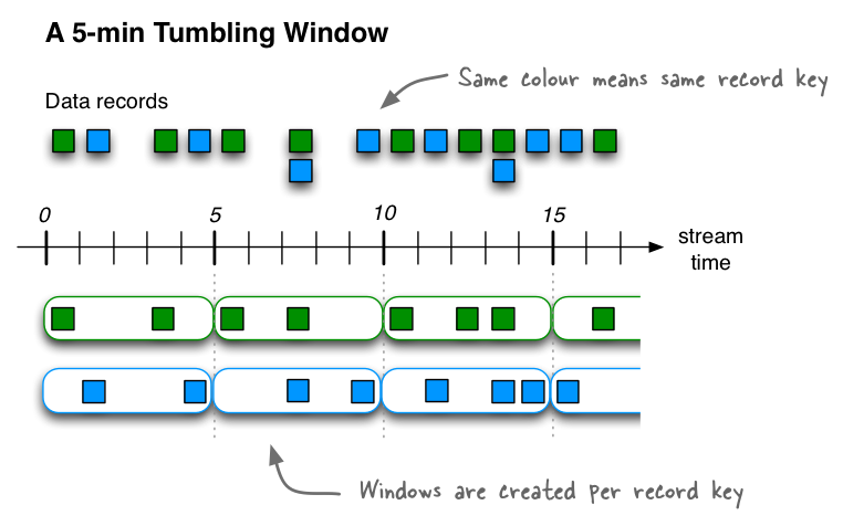
This diagram shows windowing a stream of data records with tumbling windows. Windows do not overlap because, by definition, the advance interval is identical to the window size. In this diagram the time numbers represent minutes; e.g. t=5 means “at the five-minute mark”. In reality, the unit of time in Kafka Streams is milliseconds, which means the time numbers would need to be multiplied with 60 * 1,000 to convert from minutes to milliseconds (e.g. t=5 would become t=300,000).
Tumbling time windows are aligned to the epoch, with the lower interval bound being inclusive and the upper bound
being exclusive. “Aligned to the epoch” means that the first window starts at timestamp zero. For example, tumbling
windows with a size of 5000ms have predictable window boundaries [0;5000),[5000;10000),... — and not
[1000;6000),[6000;11000),... or even something “random” like [1452;6452),[6452;11452),....
The following code defines a tumbling window with a size of 5 minutes:
import java.util.concurrent.TimeUnit;
import org.apache.kafka.streams.kstream.TimeWindows;

// A tumbling time window with a size of 5 minutes (and, by definition, an implicit
// advance interval of 5 minutes).
long windowSizeMs = TimeUnit.MINUTES.toMillis(5); // 5 * 60 * 1000L
TimeWindows.of(windowSizeMs);

// The above is equivalent to the following code:
TimeWindows.of(windowSizeMs).advanceBy(windowSizeMs);
Counting example using tumbling windows:
// Key (String) is user id, value (Avro record) is the page view event for that user.
// Such a data stream is often called a "clickstream".
KStream<String, GenericRecord> pageViews = ...;

// Count page views per window, per user, with tumbling windows of size 5 minutes
KTable<Windowed<String>, Long> windowedPageViewCounts = pageViews
    .groupByKey(Serdes.String(), genericAvroSerde)
    .count(TimeWindows.of(TimeUnit.MINUTES.toMillis(5)), "views-per-window-by-user");
Hopping time windows are windows based on time intervals. They model fixed-sized, (possibly) overlapping windows. A hopping window is defined by two properties: the window’s size and its advance interval (aka “hop”). The advance interval specifies by how much a window moves forward relative to the previous one. For example, you can configure a hopping window with a size 5 minutes and an advance interval of 1 minute. Since hopping windows can overlap – and in general they do – a data record may belong to more than one such windows.
Note
Hopping windows vs. sliding windows: Hopping windows are sometimes called “sliding windows” in other stream processing tools. Kafka Streams follows the terminology in academic literature, where the semantics of sliding windows are different to those of hopping windows.
The following code defines a hopping window with a size of 5 minutes and an advance interval of 1 minute:
import java.util.concurrent.TimeUnit;
import org.apache.kafka.streams.kstream.TimeWindows;

// A hopping time window with a size of 5 minutes and an advance interval of 1 minute.
// The window's name -- the string parameter -- is used to e.g. name the backing state store.
long windowSizeMs = TimeUnit.MINUTES.toMillis(5); // 5 * 60 * 1000L
long advanceMs =    TimeUnit.MINUTES.toMillis(1); // 1 * 60 * 1000L
TimeWindows.of(windowSizeMs).advanceBy(advanceMs);
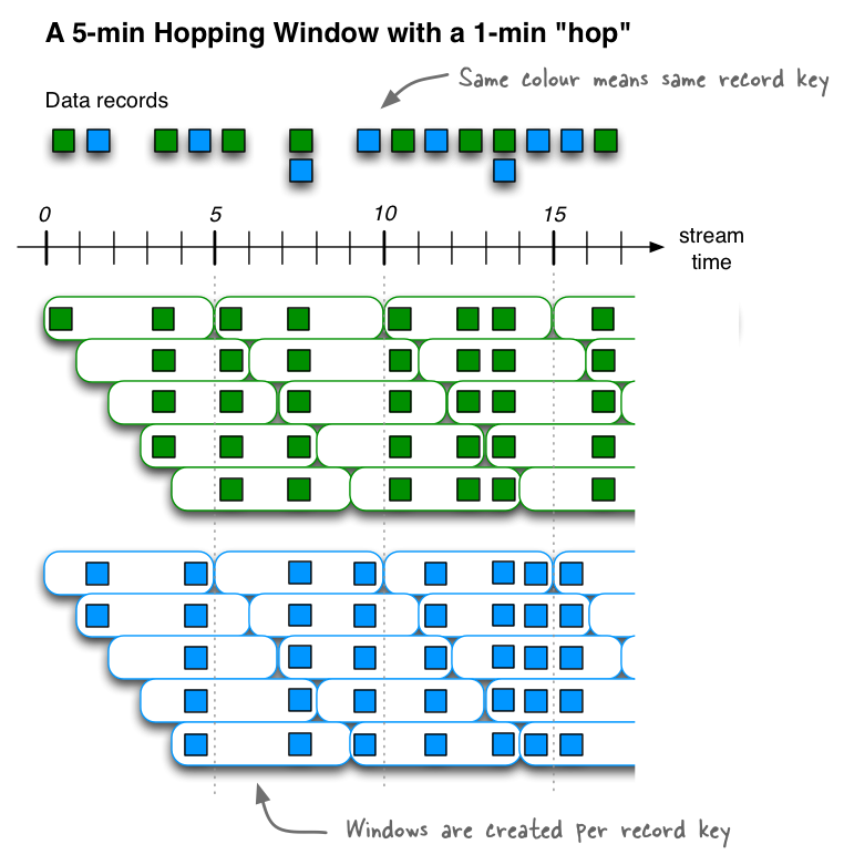
This diagram shows windowing a stream of data records with hopping windows. In this diagram the time numbers represent minutes; e.g. t=5 means “at the five-minute mark”. In reality, the unit of time in Kafka Streams is milliseconds, which means the time numbers would need to be multiplied with 60 * 1,000 to convert from minutes to milliseconds (e.g. t=5 would become t=300,000).
Hopping time windows are aligned to the epoch, with the lower interval bound being inclusive and the upper bound
being exclusive. “Aligned to the epoch” means that the first window starts at timestamp zero. For example, hopping
windows with a size of 5000ms and an advance interval (“hop”) of 3000ms have predictable window boundaries
[0;5000),[3000;8000),... — and not [1000;6000),[4000;9000),... or even something “random” like
[1452;6452),[4452;9452),....
Counting example using hopping windows:
// Key (String) is user id, value (Avro record) is the page view event for that user.
// Such a data stream is often called a "clickstream".
KStream<String, GenericRecord> pageViews = ...;

// Count page views per window, per user, with hopping windows of size 5 minutes that advance every 1 minute
KTable<Windowed<String>, Long> windowedPageViewCounts = pageViews
    .groupByKey(Serdes.String(), genericAvroSerde)
    .count(TimeWindows.of(TimeUnit.MINUTES.toMillis(5)).advanceBy(TimeUnit.MINUTES.toMillis(1)), "views-per-window-by-user");
Unlike non-windowed aggregates that we have seen previously, windowed aggregates return a windowed KTable whose keys
type is Windowed<K>. This is to differentiate aggregate values with the same key from different windows. The
corresponding window instance and the embedded key can be retrieved as Windowed#window() and Windowed#key(),
respectively.
Sliding windows are actually quite different from hopping and tumbling windows. In Kafka Streams, sliding windows
are used only for join operations, and can be specified through the
JoinWindows class.
A sliding window models a fixed-size window that slides continuously over the time axis; here, two data records are said to be included in the same window if (in the case of symmetric windows) the difference of their timestamps is within the window size. Thus, sliding windows are not aligned to the epoch, but to the data record timestamps. In contrast to hopping and tumbling windows, the lower and upper window time interval bounds of sliding windows are both inclusive.
Session windows are used to aggregate key-based events into so-called sessions, the process of which is referred to as sessionization. Sessions represent a period of activity separated by a defined gap of inactivity (or “idleness”). Any events processed that fall within the inactivity gap of any existing sessions are merged into the existing sessions. If an event falls outside of the session gap, then a new session will be created.
Session windows are different from the other window types in that:
- all windows are tracked independently across keys – e.g. windows of different keys typically have different start and end times
- their window sizes sizes vary – even windows for the same key typically have different sizes
The prime area of application for session windows is user behavior analysis. Session-based analyses can range from simple metrics (e.g. count of user visits on a news website or social platform) to more complex metrics (e.g. customer conversion funnel and event flows).
The following code defines a session window with an inactivity gap of 5 minutes:
import java.util.concurrent.TimeUnit;
import org.apache.kafka.streams.kstream.SessionWindows;

// A session window with an inactivity gap of 5 minutes.
SessionWindows.with(TimeUnit.MINUTES.toMillis(5));
Given the previous session window example, here’s what would happen on an input stream of six records. When the first three records arrive (upper part of in the diagram below), we’d have three sessions (see lower part) after having processed those records: two for the green record key, with one session starting and ending at the 0-minute mark (only due to the illustration it looks as if the session goes from 0 to 1), and another starting and ending at the 6-minute mark; and one session for the blue record key, starting and ending at the 2-minute mark.
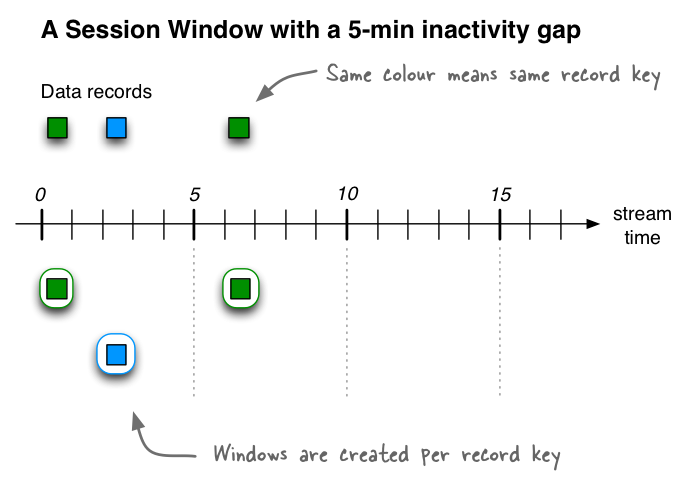
Detected sessions after having received three input records: two records for the green record key at t=0 and t=6, and one record for the blue record key at t=2. In this diagram the time numbers represent minutes; e.g. t=5 means “at the five-minute mark”. In reality, the unit of time in Kafka Streams is milliseconds, which means the time numbers would need to be multiplied with 60 * 1,000 to convert from minutes to milliseconds (e.g. t=5 would become t=300,000).
If we then receive three additional records (including two late-arriving records), what would happen is that the two existing sessions for the green record key will be merged into a single session starting at time 0 and ending at time 6, consisting of a total of three records. The existing session for the blue record key will be extended to end at time 5, consisting of a total of two records. And, finally, there will be a new session for the blue key starting and ending at time 11.
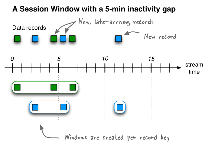
Detected sessions after having received six input records. Note the two late-arriving data records at t=4 (green) and t=5 (blue), which lead to a merge of sessions and an extension of a session, respectively.
Counting example using session windows: Let’s say we want to analyze reader behavior on a news website such as the New York Times, given a session definition of “As long as a person views (clicks on) another page at least once every 5 minutes (= inactivity gap), we consider this to be a single visit and thus a single, contiguous reading session of that person.” What we want to compute off of this stream of input data is the number of page views per session.
// Key (String) is user id, value (Avro record) is the page view event for that user.
// Such a data stream is often called a "clickstream".
KStream<String, GenericRecord> pageViews = ...;

// Count page views per session, per user, with session windows that have an inactivity gap of 5 minutes
KTable<Windowed<String>, Long> sessionizedPageViewCounts = pageViews
    .groupByKey(Serdes.String(), genericAvroSerde)
    .count(SessionWindows.with(TimeUnit.MINUTES.toMillis(5)), "views-per-session-by-user");
Applying processors and transformers (Processor API integration)
Beyond the aforementioned stateless and stateful transformations, you may also leverage the Processor API from the DSL. There are a number of scenarios where this may be helpful:
- Customization: You need to implement special, customized logic that is not or not yet available in the DSL.
- Combining ease-of-use with full flexibility where it’s needed: Even though you generally prefer to use the expressiveness of the DSL, there are certain steps in your processing that require more flexibility and tinkering than the DSL provides. For example, only the Processor API provides access to a record’s metadata such as its topic, partition, and offset information. However, you don’t want to switch completely to the Processor API just because of that.
- Migrating from other tools: You are migrating from other stream processing technologies that provide an imperative API, and migrating some of your legacy code to the Processor API was faster and/or easier than to migrate completely to the DSL right away.
| Transformation | Description |
|---|---|
Process
|
Terminal operation. Applies a This is essentially equivalent to adding the An example is available in the javadocs. |
Transform
|
Applies a Each input record is transformed into zero, one, or more output records (similar to the stateless Marks the stream for data re-partitioning:
Applying a grouping or a join after
An example is available in the javadocs. Also, a full end-to-end demo is available at MixAndMatchLambdaIntegrationTest. |
Transform (values only)
|
Applies a Each input record is transformed into exactly one output record (zero output records or multiple output records are not possible).
The
An example is available in the javadocs. |
The following example shows how to leverage, via the KStream#process() method, a custom Processor that sends an
email notification whenever a page view count reaches a predefined threshold.
First, we need to implement a custom stream processor, PopularPageEmailAlert, that implements the Processor
interface:
// A processor that sends an alert message about a popular page to a configurable email address
public class PopularPageEmailAlert implements Processor<PageId, Long> {

  private final String emailAddress;
  private ProcessorContext context;

  public PopularPageEmailAlert(String emailAddress) {
    this.emailAddress = emailAddress;
  }

  @Override
  public void init(ProcessorContext context) {
    this.context = context;

    // Here you would perform any additional initializations such as setting up an email client.
  }

  @Override
  void process(PageId pageId, Long count) {
    // Here you would format and send the alert email.
    //
    // In this specific example, you would be able to include information about the page's ID and its view count
    // (because the class implements `Processor<PageId, Long>`).
  }

  @Override
  void punctuate(long timestamp) {
    // Stays empty.  In this use case there would be no need for a periodical action of this processor.
  }

  @Override
  void close() {
    // Any code for clean up would go here.  This processor instance will not be used again after this call.
  }

}
Tip
Even though we do not demonstrate it in this example, a stream processor can access any available state stores by
calling ProcessorContext#getStateStore(). Only such state stores are available that (1) have been named in the
corresponding KStream#process() method call (note that this is a different method than Processor#process()),
plus (2) all global stores. Note that global stores do not need to be attached explicitly; however, they only
allow for read-only access.
Then we can leverage the PopularPageEmailAlert processor in the DSL via KStream#process.
In Java 8+, using lambda expressions:
KStream<String, GenericRecord> pageViews = ...;

// Send an email notification when the view count of a page reaches one thousand.
pageViews.groupByKey()
         .count("PageViewCounts")
         .filter((PageId pageId, Long viewCount) -> viewCount == 1000)
         // PopularPageEmailAlert is your custom processor that implements the
         // `Processor` interface, see further down below.
         .process(() -> new PopularPageEmailAlert("[email protected]"));
In Java 7:
// Send an email notification when the view count of a page reaches one thousand.
pageViews.groupByKey().
         .count("PageViewCounts")
         .filter(
            new Predicate<PageId, Long>() {
              public boolean test(PageId pageId, Long viewCount) {
                return viewCount == 1000;
              }
            })
         .process(
           new ProcessorSupplier<PageId, Long>() {
             public Processor<PageId, Long> get() {
               // PopularPageEmailAlert is your custom processor that implements
               // the `Processor` interface, see further down below.
               return new PopularPageEmailAlert("[email protected]");
             }
           });
Writing streams back to Kafka
Any streams and tables may be (continuously) written back to a Kafka topic. As we will describe in more detail below, the output data might be re-partitioned on its way to Kafka, depending on the situation.
| Writing to Kafka | Description |
|---|---|
To
|
Terminal operation. Write the records to a Kafka topic. (KStream details, KTable details) When to provide serdes explicitly:
Several variants of KStream<String, Long> stream = ...;
KTable<String, Long> table = ...;
// Write the stream to the output topic, using the configured default key
// and value serdes of your `StreamsConfig`.
stream.to("my-stream-output-topic");
// Same for table
table.to("my-table-output-topic");
// Write the stream to the output topic, using explicit key and value serdes,
// (thus overriding the defaults of your `StreamsConfig`).
import org.apache.kafka.common.serialization.Serdes;
stream.to(Serdes.String(), Serdes.Long(), "my-stream-output-topic");
// Same for table
table.to(Serdes.String(), Serdes.Long(), "my-table-output-topic");
Causes data re-partitioning if any of the following conditions is true:
|
Through
|
Write the records to a Kafka topic and create a new stream/table from that topic.
Essentially a shorthand for When to provide serdes explicitly:
Several variants of KStreamBuilder builder = ...;
KStream<String, Long> stream = ...;
KTable<String, Long> table = ...;
// Variant 1: Imagine that your application needs to continue reading and processing
// the records after they have been written to a topic via ``to()``. Here, one option
// is to write to an output topic, then read from the same topic by constructing a
// new stream from it, and then begin processing it (here: via `map`, for example).
stream.to("my-stream-output-topic");
KStream<String, Long> newStream = builder.stream("my-stream-output-topic").map(...);
// Variant 2 (better): Since the above is a common pattern, the DSL provides the
// convenience method ``through`` that is equivalent to the code above.
// Note that you may need to specify key and value serdes explicitly, which is
// not shown in this simple example.
KStream<String, Long> newStream = stream.through("user-clicks-topic").map(...);
// ``through`` is also available for tables
KTable<String, Long> newTable = table.through("my-table-output-topic").map(...);
Causes data re-partitioning if any of the following conditions is true:
|
Note
When you want to write to systems other than Kafka: Besides writing the data back to Kafka, you can also apply a custom processor as a stream sink at the end of the processing to, for example, write to external databases. First, doing so is not a recommended pattern – we strongly suggest to use the Kafka Connect API instead. However, if you do use such a sink processor, please be aware that it is now your responsibility to guarantee message delivery semantics when talking to such external systems (e.g., to retry on delivery failure or to prevent message duplication).
Processor API
Note
See also the Kafka Streams Javadocs for a complete list of available API functionality.
Overview
For implementing most stream processing applications, users tend to pick the DSL, which is powerful yet very expressive, i.e. many data processing use cases can be implemented in just a few lines of DSL code. The Processor API, in comparison, provides you with even more flexibility than the DSL but at the expense of requiring more manual work on the side of the application developer (read: more lines of code).
For that reason the use of the Processor API is typically reserved for scenarios such as:
- Customization: You need to implement special, customized logic that is not or not yet available in the DSL.
- Combining ease-of-use with full flexibility where it’s needed: Even though you generally prefer to use the expressiveness of the DSL, there are certain steps in your processing that require more flexibility and tinkering than the DSL provides. However, you don’t want to switch completely to the Processor API just because of that.
- Migrating from other tools: You are migrating from other stream processing technologies that provide an imperative API, and migrating some of your legacy code to the Processor API was faster and/or easier than to migrate completely to the DSL right away.
The Processor API can be used to implement both stateless as well as stateful operations, where the latter is achieved through the use of state stores.
Tip
Combining the DSL and the Processor API: You can combine the convenience of the DSL with the power and flexibility of the Processor API as described in the section Applying processors and transformers (Processor API integration).
Defining a Stream Processor
As mentioned in the Concepts section, a stream processor is a node in the processor topology that represents a single processing step. With the Processor API users can define arbitrary stream processors that processes one received record at a time, and connect these processors with their associated state stores to compose the processor topology.
Users can define their customized stream processor by implementing the Processor interface, which provides two main
API methods: process() and punctuate().
process()is called on each of the received record.punctuate()is called periodically based on elapsed stream-time (by default, stream-time is configured to represent event-time). Thus,punctuate()is purely data-driven and not related to wall-clock time (even if you useWallclockTimestampExtractor). For example, let’s assume you registered apunctuate()schedule of 10 seconds. If you were to process a stream of 60 records with consecutive timestamps from 1 (first record) to 60 seconds (last record), thenpunctuate()would be called 6 times – regardless of the time required to actually process those records; i.e.,punctuate()would be called 6 times no matter whether processing these 60 records would take a second, a minute, or an hour.
Attention
Stream-time is only advanced if all input partitions over all input topics have new data (with newer timestamps) available.
If at least one partition does not have any new data available, stream-time will not be advanced and thus punctuate() will not be triggered.
This behavior is independent of the configured timestamp extractor, i.e., using WallclockTimestampExtractor does not enable wall-clock triggering of punctuate().
The Processor interface also has an init() method, which is called by the Kafka Streams library during task construction phase. Processor instances should perform any required initialization in this method. The init() method passes in a ProcessorContext instance, which provides access to the metadata of the currently processed record, including its source Kafka topic and partition, its corresponding message offset, and further such information . This context instance can also be used to schedule the punctuation period (via ProcessorContext#schedule()) for punctuate(), to forward a new record as a key-value pair to the downstream processors (via ProcessorContext#forward()), and to commit the current processing progress (via ProcessorContext#commit()).
The following example Processor implementation defines a simple word-count algorithm:
public class WordCountProcessor implements Processor<String, String> {

  private ProcessorContext context;
  private KeyValueStore<String, Long> kvStore;

  @Override
  @SuppressWarnings("unchecked")
  public void init(ProcessorContext context) {
      // keep the processor context locally because we need it in punctuate() and commit()
      this.context = context;

      // call this processor's punctuate() method every 1000 time units.
      this.context.schedule(1000);

      // retrieve the key-value store named "Counts"
      kvStore = (KeyValueStore) context.getStateStore("Counts");
  }

  @Override
  public void process(String dummy, String line) {
      String[] words = line.toLowerCase().split(" ");

      for (String word : words) {
          Long oldValue = kvStore.get(word);
          if (oldValue == null) {
              kvStore.put(word, 1L);
          } else {
              kvStore.put(word, oldValue + 1L);
          }
      }
  }

  @Override
  public void punctuate(long timestamp) {
      KeyValueIterator<String, Long> iter = this.kvStore.all();
      while (iter.hasNext()) {
          KeyValue<String, Long> entry = iter.next();
          context.forward(entry.key, entry.value.toString());
      }
      iter.close();
      // commit the current processing progress
      context.commit();
  }

  @Override
  public void close() {
      // close the key-value store
      kvStore.close();
  }

}
Note
Stateful processing with state stores:
The WordCountProcessor defined above can not only access the currently received record in its process()
method, but can also leverage state stores to maintain processing
states to e.g. remember recently arrived records for stateful processing needs such as aggregations and joins.
See the section on state stores for further details.
In the above implementation, the following actions are performed:
- In the
init()method, schedule the punctuation every 1000 time units (the time unit is normally milliseconds, which in this example would translate to punctuation every 1 second) and retrieve the local state store by its name “Counts”. - In the
process()method, upon each received record, split the value string into words, and update their counts into the state store (we will talk about this later in this section). - In the
punctuate()method, iterate the local state store and send the aggregated counts to the downstream processor (we will talk about downstream processors later in this section), and commit the current stream state.
State Stores
Overview
To implement a stateful Processor or Transformer, you need to provide one more state stores to the processor
or transformer (stateless processors or transformers do not need state stores). State stores can be used to remember
recently received input records, to track rolling aggregates, to de-duplicate input records, and much, much more.
Another great feature of state stores is that they can be
interactively queried from other applications such as a
NodeJS-based dashboard or a microservice implemented in Scala or Go.
Because an application’s state is essential for the application to work correctly, the available state store types in Kafka Streams have fault tolerance enabled by default.
Defining and creating a State Store
You can either use one of the available store types or
implement your own custom store type.
In practice, most users leverage an existing store type via the Stores factory.
Note that, when using Kafka Streams, you normally don’t create or instantiate state stores directly in your code.
Rather, you define state stores indirectly by creating a so-called StateStoreSupplier. This supplier is used by
Kafka Streams as a factory to instantiate the actual state stores locally in application instances when and where
needed.
The following store types are available out of the box.
| Store Type | Storage Engine | Fault-tolerant? | Description |
|---|---|---|---|
Persistent
KeyValueStore<K, V> |
RocksDB | Yes (enabled by default) |
// Creating a persistent key-value store:
// here, we create a `KeyValueStore<String, Long>` named "persistent-counts".
import org.apache.kafka.streams.processor.StateStoreSupplier;
import org.apache.kafka.streams.state.Stores;

// Note: The `Stores` factory returns a supplier for the state store,
// because that's what you typically need to pass as API parameter.
StateStoreSupplier countStoreSupplier =
  Stores.create("persistent-counts")
    .withKeys(Serdes.String())
    .withValues(Serdes.Long())
    .persistent()
    .build();
See PersistentKeyValueFactory for detailed factory options. |
In-memory
KeyValueStore<K, V> |
- | Yes (enabled by default) |
// Creating an in-memory key-value store:
// here, we create a `KeyValueStore<String, Long>` named "inmemory-counts".
import org.apache.kafka.streams.processor.StateStoreSupplier;
import org.apache.kafka.streams.state.Stores;

// Note: The `Stores` factory returns a supplier for the state store,
// because that's what you typically need to pass as API parameter.
StateStoreSupplier countStoreSupplier =
  Stores.create("inmemory-counts")
    .withKeys(Serdes.String())
    .withValues(Serdes.Long())
    .inMemory()
    .build();
See InMemoryKeyValueFactory for detailed factory options. |
Fault-tolerant State Stores
In order to make state stores fault-tolerant (e.g., to recover from machine crashes) as well as to allow for state store migration without data loss (e.g., to migrate a stateful stream task from one machine to another when elastically adding or removing capacity from your application), a state store can be continuously backed up to a Kafka topic behind the scenes. We sometimes refer to this topic as the state store’s associated changelog topic or simply its changelog. In the case of a machine failure, for example, the state store and thus the application’s state can be fully restored from its changelog. You can enable or disable this backup feature for a state store, and thus its fault tolerance.
By default, persistent key-value stores are fault-tolerant. They are backed by a compacted changelog topic. The purpose of compacting this topic is to prevent the topic from growing indefinitely, to reduce the storage consumed in the associated Kafka cluster, and to minimize recovery time if a state store needs to be restored from its changelog topic.
Similarly, persistent window stores are fault-tolerant. They are backed by a topic that uses both compaction and
deletion. Using deletion in addition to compaction is required for the changelog topics of window stores because of
the structure of the message keys that are being sent to the changelog topics: for window stores, the message keys are
composite keys that include not only the “normal” key but also window timestamps. For such composite keys it would not
be sufficient to enable just compaction in order to prevent a changelog topic from growing out of bounds. With deletion
enabled, old windows that have expired will be cleaned up by Kafka’s log cleaner as the log segments expire. The
default retention setting is Windows#maintainMs() + 1 day. This setting can be overriden by specifying
StreamsConfig.WINDOW_STORE_CHANGE_LOG_ADDITIONAL_RETENTION_MS_CONFIG in the StreamsConfig.
Enable / Disable Fault Tolerance of State Stores (Store Changelogs)
You can enable or disable fault tolerance for a state store by enabling or disabling, respectively, the changelogging
of the store through enableLogging() and disableLogging().
You can also fine-tune the associated topic’s configuration if needed.
Example for disabling fault-tolerance:
import org.apache.kafka.streams.processor.StateStoreSupplier;
import org.apache.kafka.streams.state.Stores;

StateStoreSupplier countStoreSupplier = Stores.create("Counts")
            .withKeys(Serdes.String())
            .withValues(Serdes.Long())
            .persistent()
            .disableLogging() // disable backing up the store to a changelog topic
            .build();
Attention
If the changelog is disabled then the attached state store is no longer fault tolerant and it can’t have any standby replicas.
Example for enabling fault tolerance, with additional changelog-topic configuration: You can add any log config from kafka.log.LogConfig. Unrecognized configs will be ignored.
import org.apache.kafka.streams.processor.StateStoreSupplier;
import org.apache.kafka.streams.state.Stores;

Map<String, String> changelogConfig = new HashMap();
// override min.insync.replicas
changelogConfig.put("min.insyc.replicas", "1")

StateStoreSupplier countStoreSupplier = Stores.create("Counts")
            .withKeys(Serdes.String())
            .withValues(Serdes.Long())
            .persistent()
            .enableLogging(changelogConfig) // enable changelogging, with custom changelog settings
            .build();
Implementing custom State Stores
Apart from using the built-in state store types, you can also
implement your own. The primary interface to implement for the store is
org.apache.kafka.streams.processor.StateStore. Beyond that, Kafka Streams also has a few extended interfaces such
as KeyValueStore.
In addition to the actual store, you also need to provide a “factory” for the store by implementing the
org.apache.kafka.streams.processor.StateStoreSupplier interface, which Kafka Streams uses to create instances of
your store.
We provide an example state store implementation in Scala, which may serve as a starting point for your own stores:
- CMSStore (Scala) – an in-memory, fault-tolerant store that leverages a Count-Min Sketch data structure for probabilistic counting of items in an input stream. The state store supplier is implemented in CMSStoreSupplier. The backup/restore functionality of the state store and thus its fault tolerance can be enabled/disabled through configuration. The changelogging of the store is performed through CMSStoreChangeLogger.
Connecting Processors and State Stores
Now that we have defined a processor (WordCountProcessor) and the
state stores, we can now construct the processor topology by connecting these processors and state stores together by
using the TopologyBuilder instance. In addition, users can add source processors with the specified Kafka topics
to generate input data streams into the topology, and sink processors with the specified Kafka topics to generate
output data streams out of the topology.
TopologyBuilder builder = new TopologyBuilder();

// add the source processor node that takes Kafka topic "source-topic" as input
builder.addSource("Source", "source-topic")

    // add the WordCountProcessor node which takes the source processor as its upstream processor
    .addProcessor("Process", () -> new WordCountProcessor(), "Source")

    // add the count store associated with the WordCountProcessor processor
    .addStateStore(countStoreSupplier, "Process")

    // add the sink processor node that takes Kafka topic "sink-topic" as output
    // and the WordCountProcessor node as its upstream processor
    .addSink("Sink", "sink-topic", "Process");
There are several steps in the above implementation to build the topology, and here is a quick walk-through:
- A source processor node named “Source” is added to the topology using the
addSourcemethod, with one Kafka topic “source-topic” fed to it. - A processor node named “Process” with the pre-defined
WordCountProcessorlogic is then added as the downstream processor of the “Source” node using theaddProcessormethod. - A predefined persistent key-value state store is created and associated with the “Process” node, using
countStoreSupplier. - A sink processor node is then added to complete the topology using the
addSinkmethod, taking the “Process” node as its upstream processor and writing to a separate “sink-topic” Kafka topic.
In this topology, the “Process” stream processor node is considered a downstream processor of the “Source” node, and an
upstream processor of the “Sink” node. As a result, whenever the “Source” node forward a newly fetched record from
Kafka to its downstream “Process” node, WordCountProcessor#process() method is triggered to process the record and
update the associated state store; and whenever context#forward() is called in the
WordCountProcessor#punctuate() method, the aggregate key-value pair will be sent via the “Sink” processor node to
the Kafka topic “sink-topic”. Note that in the WordCountProcessor implementation, users need to refer to the
same store name “Counts” when accessing the key-value store; otherwise an exception will be thrown at runtime,
indicating that the state store cannot be found; also, if the state store itself is not associated with the processor
in the TopologyBuilder code, accessing it in the processor’s init() method will also throw an exception at
runtime, indicating the state store is not accessible from this processor.
Now that we have fully defined our processor topology in our application, we can proceed to running the Kafka Streams application.
Interactive Queries
Overview
Interactive queries let you get more from streaming than just the processing of data. This feature allows you to treat the stream processing layer as a lightweight embedded database and, more concretely, to directly query the latest state of your stream processing application, without needing to materialize that state to external databases or external storage first.
As a result, interactive queries simplify the architecture of many use cases and lead to more application-centric architectures. For example, you often no longer need to operate and interface with a separate database cluster – or a separate infrastructure team in your company that runs that cluster – to share data between a Kafka Streams application (say, an event-driven microservice) and downstream applications, regardless of whether these applications use Kafka Streams or not; they may even be applications that do not run on the JVM, e.g. implemented in Python, C/C++, or JavaScript.
The following diagrams juxtapose two architectures: the first does not use interactive queries whereas the second architecture does. It depends on the concrete use case to determine which of these architectures is a better fit – the important takeaway is that Kafka Streams and interactive queries give you the flexibility to pick and to compose the right one, rather than limiting you to just a single way.
Tip
Best of both worlds: Of course you also have the option to run hybrid architectures where, for example, your application may be queried interactively but at the same time also shares some of its results with external systems (e.g. via Kafka Connect).
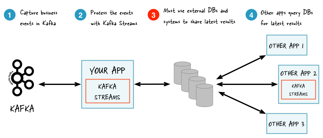
Without interactive queries: increased complexity and heavier footprint of architecture
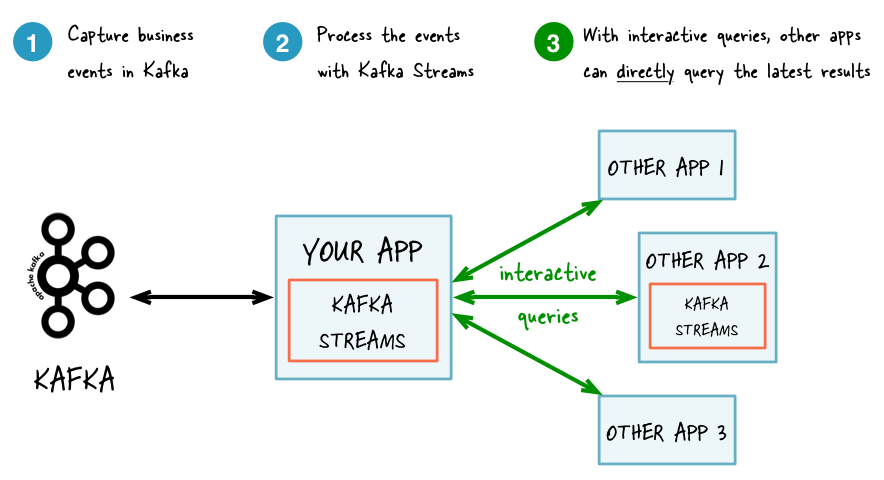
With interactive queries: simplified, more application-centric architecture
Here are some use case examples for applications that benefit from interactive queries:
- Real-time monitoring: A front-end dashboard that provides threat intelligence (e.g., web servers currently under attack by cyber criminals) can directly query a Kafka Streams application that continuously generates the relevant information by processing network telemetry data in real-time.
- Video gaming: A Kafka Streams application continuously tracks location updates from players in the gaming universe. A mobile companion app can then directly query the Kafka Streams application to show the current location of a player to friends and family, and invite them to come along. Similarly, the game vendor can use the data to identify unusual hotspots of players, which may indicate a bug or an operational issue.
- Risk and fraud: A Kafka Streams application continuously analyzes user transactions for anomalies and suspicious behavior. An online banking application can directly query the Kafka Streams application when a user logs in to deny access to those users that have been flagged as suspicious.
- Trend detection: A Kafka Streams application continuously computes the latest top charts across music genres based on user listening behavior that is collected in real-time. Mobile or desktop applications of a music store can then interactively query for the latest charts while users are browsing the store.
Demo applications
Before we explain interactive queries in detail, let us point out that we provide end-to-end demo applications to get you started:
- KafkaMusicExample: This application continuously computes the latest Top 5 music charts based on song play events collected in real-time in a Kafka topic. This charts data is maintained in a continuously updated state store that can be queried interactively via a REST API.
- WordCountInteractiveQueriesExample: This application continuously counts the occurrences of words based on text data that is consumed in real-time from a Kafka topic. The word counts are maintained in a continuously updated state store that can be queried interactively via a REST API.
Once you have familiarized yourself with the concept of interactive queries by reading the following sections, you may want to get back to the examples above and use them as a starting point for your own applications.
Your application and interactive queries
Interactive queries allow you to tap into the state of your application, and notably to do that from outside your application. However, an application is not interactively queryable out of the box: you make it queryable by leveraging the API of Kafka Streams.
It is important to understand that the state of your application – to be extra clear, we might call it “the full state of the entire application” – is typically split across many distributed instances of your application, and thus across many state stores that are managed locally by these application instances.
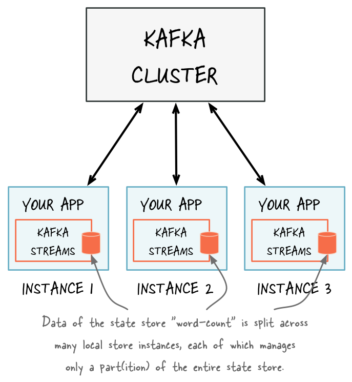
Accordingly, the API to let you interactively query your application’s state has two parts, a local and a remote one:
- Querying local state stores (for an application instance): You can query that (part of the full) state that is managed locally by an instance of your application. Here, an application instance can directly query its own local state stores. You can thus use the corresponding (local) data in other parts of your application code that are not related to calling the Kafka Streams API. Querying state stores is always read-only to guarantee that the underlying state stores will never be mutated out-of-band, e.g. you cannot add new entries; state stores should only ever be mutated by the corresponding processor topology and the input data it operates on.
- Querying remote state stores (for the entire application): To query the full state of your entire application we must be able to piece together the various local fragments of the state. In addition to being able to (a) query local state stores as described in the previous bullet point, we also need to (b) discover all the running instances of your application in the network, including their respective state stores and (c) have a way to communicate with these instances over the network, i.e. an RPC layer. Collectively, these building blocks enable intra-app communcation (between instances of the same app) as well as inter-app communication (from other applications) for interactive queries.
| What of the below is required to access the state of ... | ... an app instance (local state) | ... the entire application (full state) |
|---|---|---|
| Query local state stores of an app instance | Required (but already built-in) | Required (but already built-in) |
| Make an app instance discoverable to others | Not needed | Required (but already built-in) |
| Discover all running app instances and their state stores | Not needed | Required (but already built-in) |
| Communicate with app instances over the network (RPC) | Not needed | Required, user must provide |
Kafka Streams provides all the required functionality for interactively querying your application’s state out of the box, with but one exception: if you want to expose your application’s full state via interactive queries, then – for reasons we explain further down below – it is your responsibility to add an appropriate RPC layer (such as a REST API) to your application that allows application instances to communicate over the network. If, however, you only need to let your application instances access their own local state, then you do not need to add such an RPC layer at all.
Querying local state stores (for an application instance)
Important
A Kafka Streams application is typically running on many instances. The state that is locally available on any given instance is only a subset of the application’s entire state. Querying the local stores on an instance will, by definition, only return data locally available on that particular instance. We explain how to access data in state stores that are not locally available in section Querying remote state stores (for the entire application).
The method KafkaStreams#store(...) finds an application instance’s local state stores by name and by type.
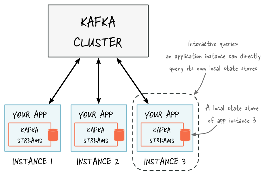
Every application instance can directly query any of its local state stores.
The name of a state store is defined when you are creating the store, either when creating the store explicitly (e.g. when using the Processor API) or when creating the store implicitly (e.g. when using stateful operations in the DSL). We show examples of how to name a state store further down below.
The type of a state store is defined by QueryableStoreType, and you can access the built-in types via the class QueryableStoreTypes.
Kafka Streams currently has two built-in types:
- A key-value store
QueryableStoreTypes#keyValueStore(), see Querying local key-value stores. - A window store
QueryableStoreTypes#windowStore(), see Querying local window stores.
Both store types return read-only versions of the underlying state stores. This read-only constraint is important to guarantee that the underlying state stores will never be mutated (e.g. new entries added) out-of-band, i.e. only the corresponding processing topology of Kafka Streams is allowed to mutate and update the state stores in order to ensure data consistency.
You can also implement your own QueryableStoreType as described in section Querying local custom state stores.
Note
Kafka Streams materializes one state store per stream partition, which means your application will potentially manage
many underlying state stores. The API to query local state stores enables you to query all of the underlying stores
without having to know which partition the data is in.
The objects returned from KafkaStreams#store(...) are therefore wrapping potentially many underlying state stores.
Querying local key-value stores
To query a local key-value store, you must first create a topology with a key-value store:
StreamsConfig config = ...;
KStreamBuilder builder = ...;
KStream<String, String> textLines = ...;

// Define the processing topology (here: WordCount)
KGroupedStream<String, String> groupedByWord = textLines
  .flatMapValues(value -> Arrays.asList(value.toLowerCase().split("\\W+")))
  .groupBy((key, word) -> word, stringSerde, stringSerde);

// Create a key-value store named "CountsKeyValueStore" for the all-time word counts
groupedByWord.count("CountsKeyValueStore");

// Start an instance of the topology
KafkaStreams streams = new KafkaStreams(builder, config);
streams.start();
Above we created a key-value store named “CountsKeyValueStore”. This store will hold the latest count for any word that is found on the topic “word-count-input”. Once the application has started we can get access to “CountsKeyValueStore” and then query it via the ReadOnlyKeyValueStore API:
// Get the key-value store CountsKeyValueStore
ReadOnlyKeyValueStore<String, Long> keyValueStore =
    streams.store("CountsKeyValueStore", QueryableStoreTypes.keyValueStore());

// Get value by key
System.out.println("count for hello:" + keyValueStore.get("hello"));

// Get the values for a range of keys available in this application instance
KeyValueIterator<String, Long> range = keyValueStore.range("all", "streams");
while (range.hasNext()) {
  KeyValue<String, Long> next = range.next();
  System.out.println("count for " + next.key + ": " + value);
}

// Get the values for all of the keys available in this application instance
KeyValueIterator<String, Long> range = keyValueStore.all();
while (range.hasNext()) {
  KeyValue<String, Long> next = range.next();
  System.out.println("count for " + next.key + ": " + value);
}
Querying local window stores
A window store differs from a key-value store in that you will potentially have many results for any given key because the key can be present in multiple windows. However, there will ever be at most one result per window for a given key.
To query a local window store, you must first create a topology with a window store:
StreamsConfig config = ...;
KStreamBuilder builder = ...;
KStream<String, String> textLines = ...;

// Define the processing topology (here: WordCount)
KGroupedStream<String, String> groupedByWord = textLines
  .flatMapValues(value -> Arrays.asList(value.toLowerCase().split("\\W+")))
  .groupBy((key, word) -> word, stringSerde, stringSerde);

// Create a window state store named "CountsWindowStore" that contains the word counts for every minute
groupedByWord.count(TimeWindows.of(60000), "CountsWindowStore");
Above we created a window store named “CountsWindowStore” that contains the counts for words in 1-minute windows. Once the application has started we can get access to “CountsWindowStore” and then query it via the ReadOnlyWindowStore API:
// Get the window store named "CountsWindowStore"
ReadOnlyWindowStore<String, Long> windowStore =
    streams.store("CountsWindowStore", QueryableStoreTypes.windowStore());

// Fetch values for the key "world" for all of the windows available in this application instance.
// To get *all* available windows we fetch windows from the beginning of time until now.
long timeFrom = 0; // beginning of time = oldest available
long timeTo = System.currentTimeMillis(); // now (in processing-time)
WindowStoreIterator<Long> iterator = windowStore.fetch("world", timeFrom, timeTo);
while (iterator.hasNext()) {
  KeyValue<Long, Long> next = iterator.next();
  long windowTimestamp = next.key;
  System.out.println("Count of 'world' @ time " + windowTimestamp + " is " + next.value);
}
Querying local custom state stores
Note
Custom state stores can only be used through the Processor API. They are not currently supported by the DSL.
Any custom state stores you use in your Kafka Streams applications can also be queried. However there are some interfaces that will need to be implemented first:
- Your custom state store must implement
StateStore. - You should have an interface to represent the operations available on the store.
- It is recommended that you also provide an interface that restricts access to read-only operations so users of this API can’t mutate the state of your running Kafka Streams application out-of-band.
- You also need to provide an implementation of
StateStoreSupplierfor creating instances of your store.
The class/interface hierarchy for your custom store might look something like:
public class MyCustomStore<K,V> implements StateStore, MyWriteableCustomStore<K,V> {
  // implementation of the actual store
}

// Read-write interface for MyCustomStore
public interface MyWriteableCustomStore<K,V> extends MyReadableCustomStore<K,V> {
  void write(K Key, V value);
}

// Read-only interface for MyCustomStore
public interface MyReadableCustomStore<K,V> {
  V read(K key);
}

public class MyCustomStoreSupplier implements StateStoreSupplier {
  // implementation of the supplier for MyCustomStore
}
To make this store queryable you need to:
- Provide an implementation of QueryableStoreType.
- Provide a wrapper class that will have access to all of the underlying instances of the store and will be used for querying.
Implementing QueryableStoreType is straight forward:
public class MyCustomStoreType<K,V> implements QueryableStoreType<MyReadableCustomStore<K,V>> {

  // Only accept StateStores that are of type MyCustomStore
  public boolean accepts(final StateStore stateStore) {
    return stateStore instanceOf MyCustomStore;
  }

  public MyReadableCustomStore<K,V> create(final StateStoreProvider storeProvider, final String storeName) {
      return new MyCustomStoreTypeWrapper(storeProvider, storeName, this);
  }

}
A wrapper class is required because even a single instance of a Kafka Streams application may run multiple stream tasks and, by doing so, manage multiple local instances of a particular state store. The wrapper class hides this complexity and lets you query a “logical” state store with a particular name without having to know about all of the underlying local instances of that state store.
When implementing your wrapper class you will need to make use of the
StateStoreProvider
interface to get access to the underlying instances of your store.
StateStoreProvider#stores(String storeName, QueryableStoreType<T> queryableStoreType) returns a List of state
stores with the given storeName and of the type as defined by queryableStoreType.
An example implemention of the wrapper follows (Java 8+):
// We strongly recommended implementing a read-only interface
// to restrict usage of the store to safe read operations!
public class MyCustomStoreTypeWrapper<K,V> implements MyReadableCustomStore<K,V> {

  private final QueryableStoreType<MyReadableCustomStore<K, V>> customStoreType;
  private final String storeName;
  private final StateStoreProvider provider;

  public CustomStoreTypeWrapper(final StateStoreProvider provider,
                                final String storeName,
                                final QueryableStoreType<MyReadableCustomStore<K, V>> customStoreType) {

    // ... assign fields ...
  }

  // Implement a safe read method
  @Override
  public V read(final K key) {
    // Get all the stores with storeName and of customStoreType
    final List<MyReadableCustomStore<K, V>> stores = provider.getStores(storeName, customStoreType);
    // Try and find the value for the given key
    final Optional<V> value = stores.stream().filter(store -> store.read(key) != null).findFirst();
    // Return the value if it exists
    return value.orElse(null);
  }

}
Putting it all together you can now find and query your custom store:
StreamsConfig config = ...;
TopologyBuilder builder = ...;
ProcessorSupplier processorSuppler = ...;

// Create CustomStoreSupplier for store name the-custom-store
MyCustomStoreSuppler customStoreSupplier = new MyCustomStoreSupplier("the-custom-store");
// Add the source topic
builder.addSource("input", "inputTopic");
// Add a custom processor that reads from the source topic
builder.addProcessor("the-processor", processorSupplier, "input");
// Connect your custom state store to the custom processor above
builder.addStateStore(customStoreSupplier, "the-processor");

KafkaStreams streams = new KafkaStreams(builder, config);
streams.start();

// Get access to the custom store
MyReadableCustomStore<String,String> store = streams.store("the-custom-store", new MyCustomStoreType<String,String>());
// Query the store
String value = store.read("key");
Querying remote state stores (for the entire application)
Typically, the ultimate goal for interactive queries is not to just query locally available state stores from within an instance of a Kafka Streams application as described in the previous section. Rather, you want to expose the application’s full state (i.e. the state across all its instances) to other applications that might be running on different machines. For example, you might have a Kafka Streams application that processes the user events in a multi-player video game, and you want to retrieve the latest status of each user directly from this application so that you can display it in a mobile companion app.
Three steps are needed to make the full state of your application queryable:
- You must add an RPC layer to your application so that the instances of your application may be interacted with via the network – notably to respond to interactive queries. By design Kafka Streams does not provide any such RPC functionality out of the box so that you can freely pick your favorite approach: a REST API, Thrift, a custom protocol, and so on. You can follow the reference examples we provide to get started with this (details further down below).
- You need to expose the respective RPC endpoints of
your application’s instances via the
application.serverconfiguration setting of Kafka Streams. Because RPC endpoints must be unique within a network, each instance will have its own value for this configuration setting. This makes an application instance discoverable by other instances. - In the RPC layer, you can then discover remote application instances and their respective state stores (e.g. for forwarding queries to other app instances if an instance lacks the local data to respond to a query) as well as query locally available state stores (in order to directly respond to queries) in order to make the full state of your application queryable.
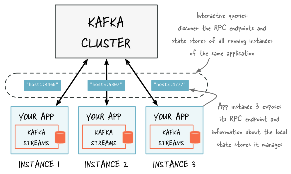
Discover any running instances of the same application as well as the respective RPC endpoints they expose for interactive queries
Adding an RPC layer to your application
As Kafka Streams doesn’t provide an RPC layer you are free to choose your favorite approach. There are many ways of doing this, and it will depend on the technologies you have chosen to use. The only requirements are that the RPC layer is embedded within the Kafka Streams application and that it exposes an endpoint that other application instances and applications can connect to.
The KafkaMusicExample and WordCountInteractiveQueriesExample are end-to-end demo applications for interactive queries that showcase the implementation of an RPC layer through a REST API.
Exposing the RPC endpoints of your application
To enable the remote discovery of state stores running within a (typically distributed) Kafka Streams application you need to set the application.server configuration property in StreamsConfig.
The application.server property defines a unique host:port pair that points to the RPC endpoint of the respective instance of a Kafka Streams application.
It’s important to understand that the value of this configuration property varies across the instances of your application.
When this property is set, then, for every instance of an application, Kafka Streams will keep track of the instance’s RPC endpoint information, its state stores, and assigned stream partitions through instances of StreamsMetadata.
Tip
You may also consider leveraging the exposed RPC endpoints of your application for further functionality, such as piggybacking additional inter-application communication that go beyond interactive queries.
Below is an example of configuring and running a Kafka Streams application that supports the discovery of its state stores.
Properties props = new Properties();
// Set the unique RPC endpoint of this application instance through which it
// can be interactively queried.  In a real application, the value would most
// probably not be hardcoded but derived dynamically.
String rpcEndpoint = "host1:4460";
props.put(StreamsConfig.APPLICATION_SERVER_CONFIG, rpcEndpoint);
// ... further settings may follow here ...

StreamsConfig config = new StreamsConfig(props);
KStreamBuilder builder = new KStreamBuilder();

KStream<String, String> textLines = builder.stream(stringSerde, stringSerde, "word-count-input");

final KGroupedStream<String, String> groupedByWord = textLines
    .flatMapValues(value -> Arrays.asList(value.toLowerCase().split("\\W+")))
    .groupBy((key, word) -> word, stringSerde, stringSerde);

// This call to `count()` creates a state store named "word-count".
// The state store is discoverable and can be queried interactively.
groupedByWord.count("word-count");

// Start an instance of the topology
KafkaStreams streams = new KafkaStreams(builder, streamsConfiguration);
streams.start();

// Then, create and start the actual RPC service for remote access to this
// application instance's local state stores.
//
// This service should be started on the same host and port as defined above by
// the property `StreamsConfig.APPLICATION_SERVER_CONFIG`.  The example below is
// fictitious, but we provide end-to-end demo applications (such as KafkaMusicExample)
// that showcase how to implement such a service to get you started.
MyRPCService rpcService = ...;
rpcService.listenAt(rpcEndpoint);
Discovering and accessing application instances and their respective local state stores
With the application.server property set, we can now find the locations of remote app instances and their state stores. The following methods return StreamsMetadata objects, which provide meta-information about application instances such as their RPC endpoint and locally available state stores.
KafkaStreams#allMetadata(): find all instances of this applicationKafkaStreams#allMetadataForStore(String storeName): find those applications instances that manage local instances of the state store “storeName”KafkaStreams#metadataForKey(String storeName, K key, Serializer<K> keySerializer): using the default stream partitioning strategy, find the one application instance that holds the data for the given key in the given state storeKafkaStreams#metadataForKey(String storeName, K key, StreamPartitioner<K, ?> partitioner): usingpartitioner, find the one application instance that holds the data for the given key in the given state store
Attention
If application.server is not configured for an application instance, then the above methods will not find any StreamsMetadata for it.
For example, we can now find the StreamsMetadata for the state store named “word-count” that we defined in the
code example shown in the previous section:
KafkaStreams streams = ...;
// Find all the locations of local instances of the state store named "word-count"
Collection<StreamsMetadata> wordCountHosts = streams.allMetadataForStore("word-count");

// For illustrative purposes, we assume using an HTTP client to talk to remote app instances.
HttpClient http = ...;

// Get the word count for word (aka key) 'alice': Approach 1
//
// We first find the one app instance that manages the count for 'alice' in its local state stores.
StreamsMetadata metadata = streams.metadataForKey("word-count", "alice", Serdes.String().serializer());
// Then, we query only that single app instance for the latest count of 'alice'.
// Note: The RPC URL shown below is fictitious and only serves to illustrate the idea.  Ultimately,
// the URL (or, in general, the method of communication) will depend on the RPC layer you opted to
// implement.  Again, we provide end-to-end demo applications (such as KafkaMusicExample) that showcase
// how to implement such an RPC layer.
Long result = http.getLong("http://" + metadata.host() + ":" + metadata.port() + "/word-count/alice");

// Get the word count for word (aka key) 'alice': Approach 2
//
// Alternatively, we could also choose (say) a brute-force approach where we query every app instance
// until we find the one that happens to know about 'alice'.
Optional<Long> result = streams.allMetadataForStore("word-count")
    .stream()
    .map(streamsMetadata -> {
        // Construct the (fictituous) full endpoint URL to query the current remote application instance
        String url = "http://" + streamsMetadata.host() + ":" + streamsMetadata.port() + "/word-count/alice";
        // Read and return the count for 'alice', if any.
        return http.getLong(url);
    })
    .filter(s -> s != null)
    .findFirst();
At this point the full state of the application is interactively queryable:
- We can discover the running instances of the application as well as the state stores they manage locally.
- Through the RPC layer that was added to the application, we can communicate with these application instances over the network and query them for locally available state.
- The application instances are able to serve such queries because they can directly query their own local state stores and respond via the RPC layer.
- Collectively, this allows us to query the full state of the entire application.
Now, if you are interested in seeing how an end-to-end application with interactive queries looks like, then we recommend to take a look at the demo applications we provide.
Memory management
Record caches in the DSL
Developers of an application using the DSL have the option to specify, for an instance of a processing topology, the
total memory (RAM) size of a record cache that is leveraged by the following KTable instances:
- Source
KTable, i.e.KTableinstances that are created viaKStreamBuilder#table()orKStreamBuilder#globalTable(). - Aggregation
KTable, i.e. instances ofKTablethat are created as a result of aggregations.
For such KTable instances, the record cache is used for:
- Internal caching and compacting of output records before they are written by the underlying stateful processor node to its internal state stores.
- Internal caching and compacting of output records before they are forwarded from the underlying stateful processor node to any of its downstream processor nodes.
Here is a motivating example:
Imagine the input is a
KStream<String, Integer>with the records<K,V>: <A, 1>, <D, 5>, <A, 20>, <A, 300>. Note that the focus in this example is on the records with key ==A.An aggregation computes the sum of record values, grouped by key, for the input above and returns a
KTable<String, Integer>.- Without caching, what is emitted for key
Ais a sequence of output records that represent changes in the resulting aggregation table (here, the parentheses denote changes, where the left and right numbers denote the new aggregate value and the previous aggregate value, respectively):<A, (1, null)>, <A, (21, 1)>, <A, (321, 21)>. - With caching, the aforementioned three output records for key
Awould likely be compacted in the cache, leading to a single output record<A, (321, null)>that is written to the aggregation’s internal state store and being forwarded to any downstream operations.
- Without caching, what is emitted for key
The cache size is specified through the cache.max.bytes.buffering parameter, which is a global setting per
processing topology:
// Enable record cache of size 10 MB.
Properties streamsConfiguration = new Properties();
streamsConfiguration.put(StreamsConfig.CACHE_MAX_BYTES_BUFFERING_CONFIG, 10 * 1024 * 1024L);
This parameter controls the number of bytes allocated for caching. Specifically, for a processor topology instance with
T threads and C bytes allocated for caching, each thread will have an even C/T bytes to construct its own
cache and use as it sees fit among its tasks. I.e., there are as many caches as there are threads, but no sharing of
caches across threads happens. The basic API for the cache is made of put() and get() calls. Records are
evicted using a simple LRU scheme once the cache size is reached. The first time a keyed record R1 = <K1, V1>
finishes processing at a node, it is marked as dirty in the cache. Any other keyed record R2 = <K1, V2> with the
same key K1 that is processed on that node during that time will overwrite <K1, V1>, which we also refer to as
“being compacted”. Note that this has the same effect as
Kafka’s log compaction, but happens (a) earlier, while the
records are still in memory, and (b) within your client-side application rather than on the server-side aka the Kafka
broker. Upon flushing R2 is (1) forwarded to the next processing node and (2) written to the local state store.
The semantics of caching is that data is flushed to the state store and forwarded to the next downstream processor node
whenever the earliest of commit.interval.ms or cache.max.bytes.buffering (cache pressure) hits. Both
commit.interval.ms and cache.max.bytes.buffering are global parameters: they apply to all processor nodes in
the topology, i.e., it is not possible to specify different parameters for each node. Below we provide some example
settings for both parameters based on desired scenarios.
To turn off caching the cache size can be set to zero:
// Disable record cache
Properties streamsConfiguration = new Properties();
streamsConfiguration.put(StreamsConfig.CACHE_MAX_BYTES_BUFFERING_CONFIG, 0);
Turning off caching might result in high write traffic for the underlying RocksDB store. With default settings caching is enabled within Kafka Streams but RocksDB caching is disabled. Thus, to avoid high write traffic it is recommended to enable RocksDB caching if Kafka Streams caching is turned off.
For example, the RocksDB Block Cache could be set to 100MB and Write Buffer size to 32 MB. See RocksDB config.
To enable caching but still have an upper bound on how long records will be cached, the commit interval can be set appropriately (in this example, it is set to 1000 milliseconds):
Properties streamsConfiguration = new Properties();
// Enable record cache of size 10 MB.
streamsConfiguration.put(StreamsConfig.CACHE_MAX_BYTES_BUFFERING_CONFIG, 10 * 1024 * 1024L);
// Set commit interval to 1 second.
streamsConfiguration.put(StreamsConfig.COMMIT_INTERVAL_MS_CONFIG, 1000);
The illustration below shows the effect of these two configurations visually. For simplicity we have records with 4 keys: blue, red, yellow and green. Without loss of generality, let’s assume the cache has space for only 3 keys. When the cache is disabled, we observer that all the input records will be output. With the cache enabled, we make the following observations. First, most records are output at the end of a commit intervals (e.g., at t1 one blue records is output, which is the final over-write of the blue key up to that time). Second, some records are output because of cache pressure, i.e. before the end of a commit interval (cf. the red record right before t2). With smaller cache sizes we expect cache pressure to be the primary factor that dictates when records are output. With large cache sizes, the commit interval will be the primary factor. Third, the number of records output has been reduced (here: from 15 to 8).
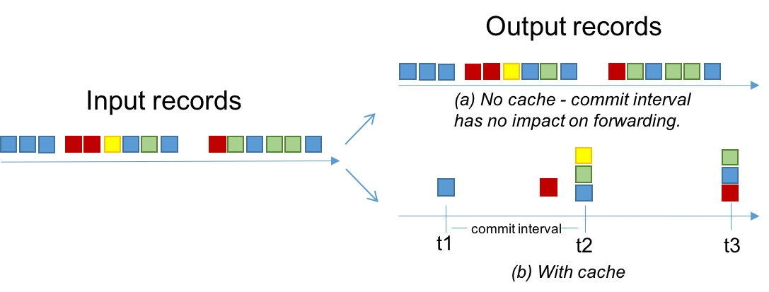
State store caches in the Processor API
Developers of a Kafka Streams application using the Processor API have the option to specify, for an instance of a processing topology, the total memory (RAM) size of the state store cache that is used for:
- Internal caching and compacting of output records before they are written from a stateful processor node to its state stores.
Note that, unlike record caches in the DSL, the state store cache in the Processor API will not cache or compact any output records that are being forwarded downstream. In other words, downstream processor nodes see all records, whereas the state stores see a reduced number of records. It is important to note that this does not impact correctness of the system but is merely a performance optimization for the state stores.
A note on terminology: we use the narrower term state store caches when we refer to the Processor API and the broader term record caches when we are writing about the DSL. We made a conscious choice to not expose the more general record caches to the Processor API so that we keep it simple and flexible. For example, developers of the Processor API might chose to store a record in a state store while forwarding a different value downstream, i.e., they might not want to use the unified record cache for both state store and forwarding downstream.
Following from the example first shown in section State Stores, to enable caching, you can
add the enableCaching call (note that caches are disabled by default and there is no explicit disableCaching
call) :
StateStoreSupplier countStoreSupplier =
  Stores.create("Counts")
    .withKeys(Serdes.String())
    .withValues(Serdes.Long())
    .persistent()
    .enableCaching()
    .build();
Other memory usage
There are other modules inside Apache Kafka that allocate memory during runtime. They include the following:
- Producer buffering, managed by the producer config
buffer.memory. - Consumer buffering, currently not strictly managed, but can be indirectly controlled by fetch size, i.e.,
fetch.max.bytesandfetch.max.wait.ms. - Both producer and consumer also have separate TCP send / receive buffers that are not counted as the buffering memory.
These are controlled by the
send.buffer.bytes/receive.buffer.bytesconfigs. - Deserialized objects buffering: after
consumer.poll()returns records, they will be deserialized to extract timestamp and buffered in the streams space. Currently this is only indirectly controlled bybuffered.records.per.partition. - RocksDB’s own memory usage, both on-heap and off-heap; critical configs (for RocksDB version 4.1.0) include
block_cache_size,write_buffer_sizeandmax_write_buffer_number. These can be specified through therocksdb.config.setterconfiguration.
Running a Kafka Streams application
In this section we describe how you can:
- Launch your application
- Elasticly add capacity to and remove capacity from your application during runtime
- Reset your application in order to reprocess its data from scratch – think: an application “reset” button
Starting a Kafka Streams application
A Java application that uses the Kafka Streams library can be run just like any other Java application – there is no special magic or requirement on the side of Kafka Streams.
For example, you can package your Java application as a fat jar file and then start the application via:
# Start the application in class `com.example.MyStreamsApp`
# from the fat jar named `path-to-app-fatjar.jar`.
$ java -cp path-to-app-fatjar.jar com.example.MyStreamsApp
The Kafka Streams examples under https://github.com/confluentinc/examples demonstrate how you can package and start your application in this way. See the README and pom.xml for details.
It is important to understand that, when starting your application as described above, you are actually launching what Kafka Streams considers to be one instance of your application. More than one instance of your application may be running at a time, and in fact the common scenario is that there are indeed multiple instances of your application running in parallel. See Parallelism Model for further information.
When the application instance starts running, the defined processor topology will be initialized as one or more stream tasks. If the processor topology defines any state stores, these state stores will also be (re-)constructed, if possible, during the initialization period of their associated stream tasks (for more details read the State restoration during workload rebalance section).
Elastic scaling of your application
Kafka Streams makes your stream processing applications elastic and scalable: you can add and remove processing capacity dynamically during the runtime of your application, and you can do so without any downtime or data loss. This means that, unlike other stream processing technologies, with Kafka Streams you do not have to completely stop your application, recompile/reconfigure, and then restart. This is great not just for intentionally adding or removing processing capacity, but also for being resilient in the face of failures (e.g. machine crashes, network outages) and for allowing maintenance work (e.g. rolling upgrades).
If you are wondering how this elasticity is actually achieved behind the scenes, you may want to read the Architecture chapter, notably the Parallelism Model section. In a nutshell, Kafka Streams leverages existing functionality in Kafka, notably its group management functionality. This group management, which is built right into the Kafka wire protocol, is the foundation that enables the elasticity of Kafka Streams applications: members of a group will coordinate and collaborate jointly on the consumption and processing of data in Kafka. On top of this foundation Kafka Streams provides some additional functionality, e.g. to enable stateful processing and to allow for fault-tolerant state in environments where application instances may come and go at any time.
Adding capacity to your application (“expand”)
If you need more processing capacity for your stream processing application, you can simply start another instance of your stream processing application, e.g. on another machine, in order to scale out. The instances of your application will become aware of each other and automatically begin to share the processing work. More specifically, what will be handed over from the existing instances to the new instances is (some of) the stream tasks that have been run by the existing instances. Moving stream tasks from one instance to another results in moving the processing work plus any internal state of these stream tasks (the state of a stream task will be re-created in the target instance by restoring the state from its corresponding changelog topic).
The various instances of your application each run in their own JVM process, which means that each instance can leverage all the processing capacity that is available to their respective JVM process (minus the capacity that any non-Kafka-Streams part of your application may be using). This explains why running additional instances will grant your application additional processing capacity. The exact capacity you will be adding by running a new instance depends of course on the environment in which the new instance runs: available CPU cores, available main memory and Java heap space, local storage, network bandwidth, and so on. Similarly, if you stop any of the running instances of your application, then you are removing and freeing up the respective processing capacity.
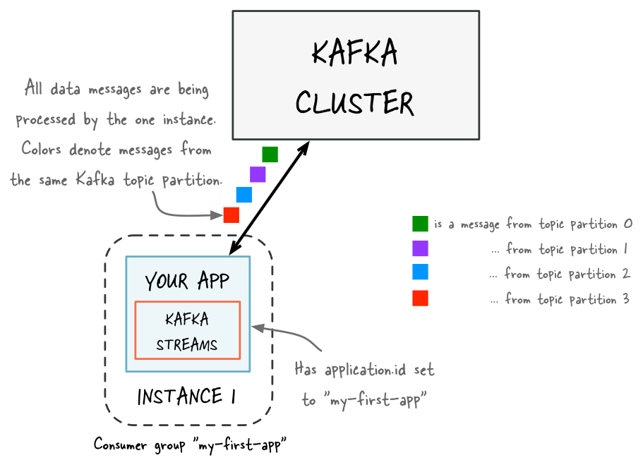
Before adding capacity: only a single instance of your Kafka Streams application is running. At this point the corresponding Kafka consumer group of your application contains only a single member (this instance). All data is being read and processed by this single instance.
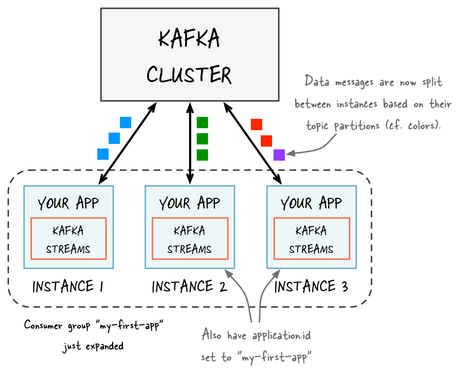
After adding capacity: now two additional instances of your Kafka Streams application are running, and they have automatically joined the application’s Kafka consumer group for a total of three current members. These three instances are automatically splitting the processing work between each other. The splitting is based on the Kafka topic partitions from which data is being read.
Removing capacity from your application (“shrink”)
If you need less processing capacity for your stream processing application, you can simply stop one or more running instances of your stream processing application, e.g. shut down 2 of 4 running instances. The remaining instances of your application will become aware that other instances were stopped and automatically take over the processing work of the stopped instances. More specifically, what will be handed over from the stopped instances to the remaining instances is the stream tasks that were run by the stopped instances. Moving stream tasks from one instance to another results in moving the processing work plus any internal state of these stream tasks (the state of a stream task will be re-created in the target instance by restoring the state from its corresponding changelog topic).
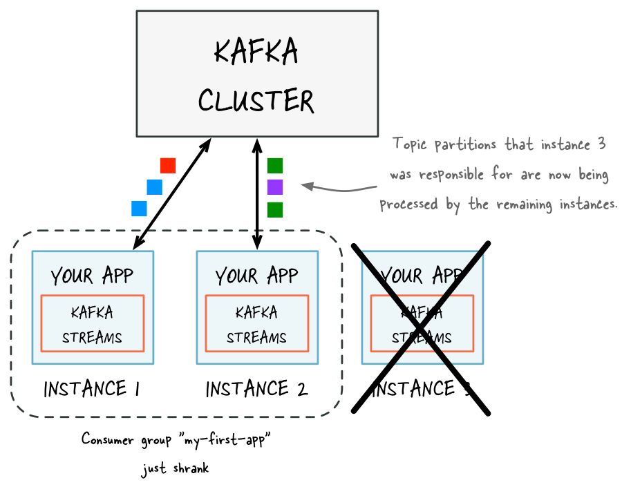
If one of the application instances is stopped (e.g. intentional reduction of capacity, maintenance, machine failure), it will automatically leave the application’s consumer group, which causes the remaining instances to automatically take over the stopped instance’s processing work.
State restoration during workload rebalance
As mentioned above, when the processing workload is rebalanced among the existing application instances either due to scaling changes (e.g. adding capacity to the application) or due to unexpected failures, some stream tasks will be migrated from one instance to another.
And when a task is migrated, the processing state of this task will be fully restored before the application instance can resume processing in order to guarantee correct processing results.
In Kafka Streams, state restoration is usually done by replaying the corresponding changelog topic to reconstruct the state store; additionally, users can also specify num.standby.replicas to minimize changelog-based restoration latency
with replicated local state stores (see Standby Replicas for more details). As a result, when the stream task is (re-)initialized on the application instance, its state store is restored in the following way:
- If no local state store exists then replay the changelog from the earliest to the current offset. In doing so, the local state store is reconstructed to the most recent snapshot.
- If a local state store exists then replay the changelog from the previously checkpointed offset. Apply the changes to restore the state state to the most recent snapshot. This will take less time as it is applying a smaller portion of the changelog.
How many application instances to run?
How many instances can or should you run for your application? Is there an upper limit for the number of instances and, similarly, for the parallelism of your application? In a nutshell, the parallelism of a Kafka Streams application – similar to the parallelism of Kafka – is primarily determined by the number of partitions of the input topic(s) from which your application is reading. For example, if your application reads from a single topic that has 10 partitions, then you can run up to 10 instances of your applications (note that you can run further instances but these will be idle).
The number of topic partitions is the upper limit for the parallelism of your Kafka Streams application and thus for the number of running instances of your application.
Tip
How to achieve a balanced processing workload across application instances to prevent processing hotpots: The balance of the processing work between application instances depends on factors such as how well data messages are balanced between partitions (think: if you have 2 topic partitions, having 1 million messages in each partition is better than having 2 million messages in the first partition and no messages in the second) and how much processing capacity is required to process the messages (think: if the time to process messages varies heavily, then it is better to spread the processing-intensive messages across partitions rather than storing these messages within the same partition).
If your data happens to be heavily skewed in the way described above, some application instances may become processing hotspots (say, when most messages would end up being stored in only 1 of 10 partitions, then the application instance that is processing this one partition would be performing most of the work while other instances might be idle). You can minimize the likelihood of such hotspots by ensuring better data balancing across partitions (i.e. minimizing data skew at the point in time when data is being written to the input topics in Kafka) and by over-partitioning the input topics (think: use 50 or 100 partitions instead of just 10), which lowers the probability that a small subset of partitions will end up storing most of the topic’s data.
Application Reset Tool
Overview
The Application Reset Tool allows you to quickly reset an application in order to reprocess its data from scratch – think: an application “reset” button.
Scenarios when would you like to reset an application include:
- Development and testing
- Addressing bugs in production
- Demos
However, resetting an application manually is a bit involved. Kafka Streams is designed to hide many details about operator state, fault-tolerance, and internal topic management from the user (especially when using Kafka Streams DSL). In general this hiding of details is very desirable but it also makes manually resetting an application more difficult. The Application Reset Tool fills this gap and allows you to quickly reset an application.
Scope
As mentioned in section Managing topics of a Kafka Streams application, there are two different categories of topics in Kafka Streams: user topics (input, output, and intermediate topics) and internal topics. The application reset tool treats these topics differently when resetting the application.
What the application reset tool does:
- For any specified input topics:
- Reset to the beginning of the topic, i.e., set the application’s committed consumer offsets for all partitions
to each partition’s
earliestoffset (for consumer groupapplication.id).
- Reset to the beginning of the topic, i.e., set the application’s committed consumer offsets for all partitions
to each partition’s
- For any specified intermediate topics:
- Skip to the end of the topic, i.e., set the application’s committed consumer offsets for all partitions to each
partition’s
logSize(for consumer groupapplication.id).
- Skip to the end of the topic, i.e., set the application’s committed consumer offsets for all partitions to each
partition’s
- For any internal topics:
- Delete the internal topic (this automatically deletes any committed offsets).
What the application reset tool does not:
- Does not reset output topics of an application. If any output (or intermediate) topics are consumed by downstream applications, it is your responsibility to adjust those downstream applications as appropriate when you reset the upstream application.
- Does not reset the local environment of your application instances. It is your responsibility to delete the local state on any machine on which an application instance was run. See the instructions in section Step 2: Reset the local environments of your application instances on how to do this.
Usage
Step 1: Run the application reset tool
Attention
Use this tool only if the application is fully stopped:
You must use this script only if no instances of your application are running.
Otherwise the application may enter an invalid state, crash, or produce incorrect results.
You can check if the consumer group with ID application.id is still active using bin/kafka-consumer-groups.
Use this tool with care and double-check its parameters:
If you provide wrong parameter values (e.g. typos in application.id) or specify
parameters inconsistently (e.g. specifying the wrong input topics for the application),
this tool might invalidate the application’s state or even impact other applications,
consumer groups, or Kafka topics of your Kafka cluster.
You can call the application reset tool on the command line via bin/kafka-streams-application-reset.
The tool accepts the following parameters:
Option (* = required)         Description
---------------------         -----------
* --application-id <id>       The Kafka Streams application ID (application.id)
--bootstrap-servers <urls>    Comma-separated list of broker urls with format: HOST1:PORT1,HOST2:PORT2
                                (default: localhost:9092)
--intermediate-topics <list>  Comma-separated list of intermediate user topics
--input-topics <list>         Comma-separated list of user input topics
--zookeeper <url>             Format: HOST:POST
                                (default: localhost:2181)
You can combine the parameters of the script as needed. For example, if an application should only restart from an
empty internal state but not reprocess previous data, simply omit the parameters --input-topics and
--intermediate-topics.
Tip
On intermediate topics: In general, we recommend to manually delete and re-create any intermediate topics before running the application reset tool. This allows to free disk space in Kafka brokers early on. It is important to first delete and re-create intermediate topics before running the application reset tool.
Not deleting intermediate topics and only using the application reset tool is preferable:
- when there are external downstream consumers for the application’s intermediate topics
- during development, where manually deleting and re-creating intermediate topics might be cumbersome and often unnecessary
Step 2: Reset the local environments of your application instances
Running the application reset tool (step 1) ensures that your application’s state – as tracked globally in the application’s configured Kafka cluster – is reset. However, by design the reset tool does not modify or reset the local environment of your application instances, which includes the application’s local state directory.
For a complete application reset you must also delete the application’s local state directory on
any machines on which an application instance was run prior to restarting an application instance on the same
machines. You can either use the API method KafkaStreams#cleanUp() in your application code or manually delete the
corresponding local state directory (default location: /var/lib/kafka-streams/<application.id>, cf.
state.dir configuration parameter).
Example
Let’s imagine you are developing and testing an application locally and want to iteratively improve your application via run-reset-modify cycles. You might have code such as the following:
package io.confluent.examples.streams;

import ...;

public class ResetDemo {

  public static void main(String[] args) throws Exception {
    // Kafka Streams configuration
    Properties streamsConfiguration = new Properties();
    streamsConfiguration.put(StreamsConfig.APPLICATION_ID_CONFIG, "my-streams-app");
    // ...and so on...

    // Define the processing topology
    KStreamBuilder builder = new KStreamBuilder();
    builder.stream("my-input-topic")
        .selectKey(...)
        .through("rekeyed-topic")
        .countByKey("global-count")
        .to("my-output-topic");

    KafkaStreams app = new KafkaStreams(builder, streamsConfiguration);

    // Delete the application's local state.
    // Note: In real application you'd call `cleanUp()` only under
    // certain conditions.  See tip on `cleanUp()` below.
    app.cleanUp();

    app.start();

    // Note: In real applications you would register a shutdown hook
    // that would trigger the call to `app.close()` rather than
    // using the sleep-then-close example we show here.
    Thread.sleep(30 * 1000L);
    app.close();
  }

}
Tip
Calling cleanUp() is safe but do so judiciously:
It is always safe to call KafkaStreams#cleanUp() because the local state of an application instance can be
recovered from the underlying internal changelog topic(s).
However, to avoid the corresponding recovery overhead it is recommended to not call cleanUp() unconditionally
and every time an application instance is restarted/resumed. A production application would therefore use e.g.
command line arguments to enable/disable the cleanUp() call as needed.
You can then perform run-reset-modify cycles as follows:
# Run your application
$ bin/kafka-run-class io.confluent.examples.streams.ResetDemo

# After stopping all application instances, reset the application
$ bin/kafka-streams-application-reset --application-id my-streams-app \
                                      --input-topics my-input-topic \
                                      --intermediate-topics rekeyed-topic

# Now you can modify/recompile as needed and then re-run the application again.
# You can also experiment, for example, with different input data without
# modifying the application.
Managing topics of a Kafka Streams application
Overview
A Kafka Streams application executes by continuously reading from some Kafka topics, processing the read data, and then (typically) writing the processing results back into Kafka topics. In addition, the application itself may also auto-create some other Kafka topics in the Kafka brokers such as state store changelogs topics. Therefore it is important to understand the difference between these topics and how the topics can be managed along with the your applications.
In Kafka Streams, we distinguish between user topics and internal topics. Both kinds are normal Kafka topics, but they are used differently and, in the case of internal topics, follow a specific naming convention.
User topics
User topics are topics that exist externally to an application and that will be read from or written to by the application, including:
- Input topics: topics that are specified via source processors in the application’s topology; e.g. via
KStreamBuilder#stream(),KStreamBuilder#table()andTopologyBuilder#addSource(). - Output topics: topics that are specified via sink processors in the application’s topology; e.g. via
KStream#to(),KTable.to()andTopologyBuilder#addSink(). - Intermediate topics: topics that are both input and output topics of the application’s topology; e.g. via
KStream#through().
In practice, all user topics must be created and managed manually ahead of time (e.g., via the topic tools). Note that in some cases these topics may be shared among multiple applications for reading and writing, in which case application users need to coordinate on managing such topics; in some other cases these topics are managed in a centralized way (e.g., by the team who operates the Kafka broker clusters) and application users then would not need to manage topics themselves but simply obtain access to them.
Note
Auto-creation of topics is strongly discouraged:
It is strongly recommended to NOT rely on the broker-side topic auto-creation feature to create user topics.
First, auto-creation of topics may be disabled in your Kafka cluster. Second, auto-creation will always
apply the default topic settings such as the replicaton factor, and these default settings might not be what you want
for certain output topics (cf. auto.create.topics.enable=true in the
Kafka broker configuration).
Internal topics
Internal topics are topics that are used internally by the Kafka Streams application while executing, for example, the changelog topics for state stores. Such topics are created by the application under the hood, and exclusively used by that stream application only.
If security is enabled on the Kafka brokers, users need to set the corresponding security configs to authorize the underlying clients with corresponding admin functionality to be able to create such topics (details can be found in section Security).
Note
Implementation detail on internal topic naming:
Internal topics currently follow the naming convention <application.id>-<operatorName>-<suffix>, but this convention
is not guaranteed for future releases.
Data types and serialization
Overview
Every Kafka Streams application must provide serializers and deserializers – abbreviated as serdes – for the data types of record keys and record values (e.g. java.lang.String or Avro objects) to materialize the data when necessary. Operations that require such serde information include: stream(), table(), to(), through(), groupByKey(), groupBy().
There are two ways to provide these serdes:
- By setting default serdes via a
StreamsConfiginstance. - By specifying explicit serdes when calling the appropriate API methods, thus overriding the defaults.
Configuring default serializers/deserializers (serdes)
Serdes specified in the Streams configuration via StreamsConfig are used as the default in your Kafka Streams application.
import org.apache.kafka.common.serialization.Serdes;
import org.apache.kafka.streams.StreamsConfig;

Properties settings = new Properties();
// Default serde for keys of data records (here: built-in serde for String type)
settings.put(StreamsConfig.KEY_SERDE_CLASS_CONFIG, Serdes.String().getClass().getName());
// Default serde for values of data records (here: built-in serde for Long type)
settings.put(StreamsConfig.VALUE_SERDE_CLASS_CONFIG, Serdes.Long().getClass().getName());

StreamsConfig config = new StreamsConfig(settings);
Overriding default serializers/deserializers (serdes)
You can also specify serdes explicitly by passing them to the appropriate API methods, which overrides the default serde settings:
import org.apache.kafka.common.serialization.Serde;
import org.apache.kafka.common.serialization.Serdes;

final Serde<String> stringSerde = Serdes.String();
final Serde<Long> longSerde = Serdes.Long();

// The stream userCountByRegion has type `String` for record keys (for region)
// and type `Long` for record values (for user counts).
KStream<String, Long> userCountByRegion = ...;
userCountByRegion.to(stringSerde, longSerde, "RegionCountsTopic");
If you want to override serdes selectively, i.e., keep the defaults for some fields, then pass null whenever you want to leverage the default serde settings:
import org.apache.kafka.common.serialization.Serde;
import org.apache.kafka.common.serialization.Serdes;

// Use the default serializer for record keys (here: region as String) by passing `null`,
// but override the default serializer for record values (here: userCount as Long).
final Serde<Long> longSerde = Serdes.Long();
KStream<String, Long> userCountByRegion = ...;
userCountByRegion.to(null, longSerde, "RegionCountsTopic");
Available serializers/deserializers (serdes)
Apache Kafka includes several built-in serde implementations in its kafka-clients maven artifact:
<dependency>
    <groupId>org.apache.kafka</groupId>
    <artifactId>kafka-clients</artifactId>
    <version>0.10.2.1-cp1</version>
</dependency>
This artifact provides the following serde implementations under the package org.apache.kafka.common.serialization, which you can leverage when e.g., defining default serializers in your Streams configuration.
| Data type | Serde |
|---|---|
| byte[] | Serdes.ByteArray(), Serdes.Bytes() (see tip below) |
| ByteBuffer | Serdes.ByteBuffer() |
| Double | Serdes.Double() |
| Integer | Serdes.Integer() |
| Long | Serdes.Long() |
| String | Serdes.String() |
Tip
Bytes is a wrapper for Java’s byte[] (byte array) that supports proper equality and ordering semantics. You may want to consider using Bytes instead of byte[] in your applications.
You would use the built-in serdes as follows, using the example of the String serde:
// When configuring the default serdes of StreamConfig
Properties streamsConfiguration = new Properties();
streamsConfiguration.put(StreamsConfig.KEY_SERDE_CLASS_CONFIG,   Serdes.String().getClass().getName());
streamsConfiguration.put(StreamsConfig.VALUE_SERDE_CLASS_CONFIG, Serdes.String().getClass().getName());

// When you want to override serdes explicitly/selectively
final Serde<String> stringSerde = Serdes.String();
KStreamBuilder builder = new KStreamBuilder();
KStream<String, String> textLines = builder.stream(stringSerde, stringSerde, "TextLinesTopic");
The code examples of Kafka Streams also include a basic serde implementation for JSON:
- JSON example: JsonPOJOSerializer and JsonPOJODeserializer, which you can use to construct a unified JSON serde via
Serdes.serdeFrom(<serializer>, <deserializer>)(see PageViewTypedDemo for a demonstration)
Lastly, the Confluent examples repository includes basic serde implementations for Apache Avro:
- Generic Avro serde: GenericAvroSerde
- Specific Avro serde: SpecificAvroSerde
As well as templated serde implementations:
Windowed<T>serde: WindowedSerde- PriorityQueue serde (example): PriorityQueueSerde
Implementing custom serializers/deserializers (serdes)
If you need to implement custom serdes, your best starting point is to take a look at the source code references of existing serdes (see previous section). Typically, your workflow will be similar to:
- Write a serializer for your data type
Tby implementing org.apache.kafka.common.serialization.Serializer. - Write a deserializer for
Tby implementing org.apache.kafka.common.serialization.Deserializer. - Write a serde for
Tby implementing org.apache.kafka.common.serialization.Serde, which you either do manually (see existing serdes in the previous section) or by leveraging helper functions in Serdes such asSerdes.serdeFrom(Serializer<T>, Deserializer<T>).
Security
Overview
Kafka Streams can help you make your stream processing applications secure, and it achieves this through its native integration with Kafka’s security functionality. In general, Kafka Streams supports all the client-side security features in Kafka. The most important aspect to understand is that Kafka Streams leverages Kafka’s Java Producer and Consumer API behind the scenes. Hence what you need to do to secure your stream processing applications on the side of Kafka Streams is to configure the appropriate security settings of the corresponding Kafka producer/consumer clients. Once you know which client-side security features you want to use, you simply need to include the corresponding settings in the configuration of your Kafka Streams application (see the security example below).
Note
Security features are optional: The security features in Apache Kafka are optional, and it is up to you to decide whether to enable or disable any of them. And you can mix and match these security features as needed: both secured and non-secured Kafka clusters are supported, as well as a mix of authenticated, unauthenticated, encrypted and non-encrypted clients. This flexibility allows you to model the security functionality in Kafka to match your specific needs, and to make effective cost vs. benefit (read: security vs. convenience/agility) tradeoffs: tighter security requirements in places where security matters (e.g. production), and relaxed requirements in other situations (e.g. development, testing).
In this section we will not cover these client-side security features in full detail, so we recommend reading the Kafka Security chapter (see also the Confluent blog post Apache Kafka Security 101) to familiarize yourself with the security features that are currently available in Apache Kafka. That said, let us highlight a couple of important client-side security features:
- Encrypting data-in-transit between your applications and Kafka brokers: You can enable the encryption of the client-server communication between your applications and the Kafka brokers.
- Example: You can configure your applications to always use encryption when reading data from Kafka and when writing data to Kafka; this is very important when reading/writing data across security domains (e.g. internal network vs. public Internet or partner network).
- Client authentication: You can enable client authentication for connections from your application to Kafka brokers.
- Example: You can define that only some specific applications are allowed to connect to your production Kafka cluster.
- Client authorization: You can enable client authorization of read/write operations by your applications.
- Example: You can define that only some specific applications are allowed to read from a Kafka topic that stores sensitive data. Similarly, you can restrict write access to certain Kafka topics to only a few applications to prevent e.g. data pollution or fraudulent activities.
Notable ACL settings
When you run your application against a secured Kafka cluster, you must make sure that the principal running the
application has the ACL --cluster --operation Create set so that the application has the permissions to create
internal topics.
Security example
The following example is based on the Confluent blog post Apache Kafka Security 101. What we want to do is to configure a Kafka Streams application to (a) enable client authentication and (b) encrypt data-in-transit when communicating with its Kafka cluster.
Tip
A complete demo application including step-by-step instructions is available at SecureKafkaStreamsExample.java under https://github.com/confluentinc/examples.
Because we want to focus this example on the side of Kafka Streams, we assume that (1) the security setup of the Kafka brokers in the cluster is already completed, and (2) the necessary SSL certificates are available to the application in the local filesystem locations specified below (the aforementioned blog post walks you through the steps to generate them); for example, if you are using Docker to containerize your applications, then you must also include these SSL certificates in the right locations within the Docker image.
Once these two assumptions are met, you must only configure the corresponding settings for the Kafka clients in your application. The configuration snippet below shows the settings to (a) enable client authentication and (b) enable SSL encryption for data-in-transit between your Kafka Streams application and the Kafka cluster it is reading from and writing to:
# Essential security settings to enable client authentication and SSL encryption
bootstrap.servers=kafka.example.com:9093
security.protocol=SSL
ssl.truststore.location=/etc/security/tls/kafka.client.truststore.jks
ssl.truststore.password=test1234
ssl.keystore.location=/etc/security/tls/kafka.client.keystore.jks
ssl.keystore.password=test1234
ssl.key.password=test1234
Within an application, you’d use code such as the following to configure these settings in your StreamsConfig
instance (see section Configuring a Kafka Streams application):
// Code of your Java application that uses the Kafka Streams library
Properties settings = new Properties();
settings.put(StreamsConfig.APPLICATION_ID_CONFIG, "secure-kafka-streams-app");
// Where to find secure Kafka brokers.  Here, it's on port 9093.
settings.put(StreamsConfig.BOOTSTRAP_SERVERS_CONFIG, "kafka.example.com:9093");
//
// ...further non-security related settings may follow here...
//
// Security settings.
// 1. These settings must match the security settings of the secure Kafka cluster.
// 2. The SSL trust store and key store files must be locally accessible to the application.
settings.put(CommonClientConfigs.SECURITY_PROTOCOL_CONFIG, "SSL");
settings.put(SslConfigs.SSL_TRUSTSTORE_LOCATION_CONFIG, "/etc/security/tls/kafka.client.truststore.jks");
settings.put(SslConfigs.SSL_TRUSTSTORE_PASSWORD_CONFIG, "test1234");
settings.put(SslConfigs.SSL_KEYSTORE_LOCATION_CONFIG, "/etc/security/tls/kafka.client.keystore.jks");
settings.put(SslConfigs.SSL_KEYSTORE_PASSWORD_CONFIG, "test1234");
settings.put(SslConfigs.SSL_KEY_PASSWORD_CONFIG, "test1234");
StreamsConfig streamsConfiguration = new StreamsConfig(settings);
With these settings in place your Kafka Streams application will encrypt any data-in-transit that is being read from or written to Kafka, and it will also authenticate itself against the Kafka brokers that it is talking to. (Note that this simple example does not cover client authorization.)
When things go wrong (e.g. wrong password): What would happen if you misconfigured the security settings in your
application? In this case, the application would fail at runtime, typically right after you started it. For example,
if you entered an incorrect password for the ssl.keystore.password setting, then error messages similar to the
following would be logged, and after that the application would terminate:
# Misconfigured ssl.keystore.password
Exception in thread "main" org.apache.kafka.common.KafkaException: Failed to construct kafka producer
[...snip...]
Caused by: org.apache.kafka.common.KafkaException: org.apache.kafka.common.KafkaException:
   java.io.IOException: Keystore was tampered with, or password was incorrect
[...snip...]
Caused by: java.security.UnrecoverableKeyException: Password verification failed
Tip
You can monitor the application log files of your Kafka Streams applications for such error messages to spot any misconfigured applications quickly.