|
GraphLab: Distributed Graph-Parallel API
2.1
|
|
GraphLab: Distributed Graph-Parallel API
2.1
|
The graph analytics toolkit contains applications for performing graph analytics and extracting patterns from the graph structure.
The toolkit current contains:
All toolkits take any of the graph formats described in Graph File Formats .
This is primarily a utility program, providing conversion between any of the Portable Graph formats described in Graph File Formats.
To run:
> ./format_convert --ingraph=[input graph location] --informat=[input format type]
                   --outgraph=[output graph location] --outformat[output format type]
The output is by default gzip compressed. To disable, add the option,
--outgzip=0
This program can also run distributed by using
> mpiexec -n [N machines] --hostfile [host file] ./format_convert ....
See your MPI documentation for details on how to launch this job. All machines must have access to the input graph location and the output graph location. Graphs may be on HDFS. If you have problems loading HDFS files, see the FAQ.
The undirected triangle counting program can count the total number of triangles in a graph, and can also, with little more time, count the number of triangles passing through each vertex in the graph.
It implements the edge-iterator algorithm described in
T. Schank. Algorithmic Aspects of Triangle-Based Network Analysis. Phd in computer science, University Karlsruhe, 2007.
with several optimizations.
The input to the system is a graph in any of the Portable graph format described in Graph File Formats. It is important that the input be "cleaned" and that reverse edges are removed: i.e. if edge 1–>5 exists, edge 5–>1 should not exist. (The program will run without these edge removed. But numbers may be erroneous).
To count the total number of triangles in a graph, the minimal set of options required are:
> ./undirected_triangle_count --graph=[graph prefix] --format=[format]
Output looks like:
Number of vertices: 875713
Number of edges:    4322051
Counting Triangles...
INFO:     synchronous_engine.hpp(start:1213): 0: Starting iteration: 0
INFO:     synchronous_engine.hpp(start:1257):   Active vertices: 875713
INFO:     synchronous_engine.hpp(start:1307):    Running Aggregators
Counted in 1.16463 seconds
13391903 Triangles
To count the number of triangles on each vertex, the minimal set of options are:
> ./undirected_triangle_count --graph=[graph prefix] --format=[format] --per_vertex=[output prefix]
Tne output prefix is where the output counts will be written. This may be located on HDFS. For instance, if the output_prefix is "v_out", the output files will be written to:
v_out_1_of_16
v_out_2_of_16
...
v_out_16_of_16
Each line in the output file contains two numbers: a Vertex ID, and the number of triangles intersecting the vertex.
This program can also run distributed by using
> mpiexec -n [N machines] --hostfile [host file] ./undirected_triangle_count ....
See your MPI documentation for details on how to launch this job. All machines must have access to the input graph location and the output graph location. Graphs may be on HDFS. If you have problems loading HDFS files, see the FAQ.
Relevant options are:
The directed triangle counting program counts the total number of directed triangles in a graph of each type, and can also output the number of triangles of each type passing through each vertex in the graph.
We show the 4 possible types of triangles here: In each case, the vertex being evaluated is the green vertex labeled "A". A dotted edge means that the direction of the edge do not matter.
| Triangle Name | Triangle Pattern |
|---|---|
| In Triangle | 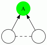
|
| Out Triangle | 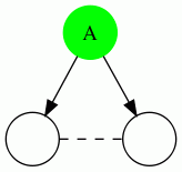
|
| Through Triangle | 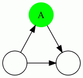
|
| Cycle Triangle | 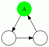
|
The input to the system is a graph in any of the Portable graph format described in Graph File Formats.
To count the total number of triangles in a graph, the minimal set of options required are:
> ./directed_triangle_count --graph=[graph prefix] --format=[format]
Output looks like this:
Number of vertices: 875713
Number of edges:    5105039
Counting Triangles...
INFO:     synchronous_engine.hpp(start:1213): 0: Starting iteration: 0
INFO:     synchronous_engine.hpp(start:1257):   Active vertices: 875713
INFO:     synchronous_engine.hpp(start:1307):    Running Aggregators
Counted in 1.962 seconds
Collecting results ...
INFO:     synchronous_engine.hpp(start:1213): 0: Starting iteration: 0
INFO:     synchronous_engine.hpp(start:1257):   Active vertices: 875713
INFO:     synchronous_engine.hpp(start:1307):    Running Aggregators
28198954 In triangles
28198954 Out triangles
28198954 Through triangles
11669313 Cycle triangles
Observe that the number of In, Out and Through triangles are identical. This is because every In-triangle necessarily forms one Out and one Through triangle, (and similarly for the rest). Also the number of Cycle Triangles must be divisible by 3 since every cycle is counted 3 times, once on each vertex in the cycle.
To count the number of triangles on each vertex, the minimal set of options are:
> ./directed_triangle_count --graph=[graph prefix] --format=[format] --per_vertex=[output prefix]
Tne output prefix is where the output counts will be written. This may be located on HDFS. For instance, if the output_prefix is "v_out", the output files will be written to:
v_out_1_of_16
v_out_2_of_16
...
v_out_16_of_16
Each line in the output file has the following format:
[vid] [in triangles] [out triangles] [through triangles] [cycle_triangles] [#out edges] [#in edges]
This program can also run distributed by using
> mpiexec -n [N machines] --hostfile [host file] ./directed_triangle_count ....
See your MPI documentation for details on how to launch this job. All machines must have access to the input graph location and the output graph location. Graphs may be on HDFS. If you have problems loading HDFS files, see the FAQ.
Relevant options are:
The PageRank program computes the pagerank of each vertex. See the Wikipedia article for details of the algorithm.
The input to the system is a graph in any of the Portable graph format described in Graph File Formats.
> ./pagerank --graph=[graph prefix] --format=[format]
Alternatively, a synthetic power law graph of an arbitrary number of vertices can be generated using:
> ./pagerank --powerlaw=[nvertices]
The resultant graph will have powerlaw out-degree, and nearly constant in-degree. The actual generation process draws vertex degree from a truncated power-law distribution with alpha=2.1. The distribution is truncated at maximum out-degree 100M to avoid allocating massive amounts of memory for creating the sampling distribution.
There are several modes of computation that are supported. All will eventually obtain the same solutions.
To get classical PageRank iterations, adding the option
> --iterations=[N Iterations]
The dynamic synchronous computation only performs computation on vertices that have not yet converged to the desired tolerance. The default tolerance is 0.001. This can be modified by adding the option
> --tol=[tolerance]
The dynamic asynchronous computation only performs computation on vertices that have not yet converged to the desired tolerance. This uses the asynchronous engine. The default tolerance is 0.001. This can be modified by adding the option
> --tol=[tolerance]
To save the resultant pagerank of each vertex, include the option
> --saveprefix=[output prefix]
Tne output prefix is where the output counts will be written. This may be located on HDFS. For instance, if the output_prefix is "v_out", the output files will be written to:
v_out_1_of_16
v_out_2_of_16
...
v_out_16_of_16
Each line in the output file contains two numbers: a Vertex ID, and the computed PageRank.
This program can also run distributed by using
> mpiexec -n [N machines] --hostfile [host file] ./pagerank ....
See your MPI documentation for details on how to launch this job. All machines must have access to the input graph location and the output graph location. Graphs may be on HDFS. If you have problems loading HDFS files, see the FAQ.
Relevant options are:
This program iteratively finds the KCore of the network.
The input to the system is a graph in any of the Portable graph format described in Graph File Formats.
> ./kcore --graph=[graph prefix] --format=[format]
Output may look like:
K=0:  #V = 875713   #E = 4322051
INFO:     synchronous_engine.hpp(start:1213): 0: Starting iteration: 0
INFO:     synchronous_engine.hpp(start:1257):   Active vertices: 0
K=1:  #V = 875713   #E = 4322051
INFO:     synchronous_engine.hpp(start:1213): 0: Starting iteration: 0
INFO:     synchronous_engine.hpp(start:1257):   Active vertices: 153407
INFO:     synchronous_engine.hpp(start:1307):    Running Aggregators
K=2:  #V = 711870   #E = 4160100
INFO:     synchronous_engine.hpp(start:1213): 0: Starting iteration: 0
INFO:     synchronous_engine.hpp(start:1257):   Active vertices: 108715
INFO:     synchronous_engine.hpp(start:1307):    Running Aggregators
K=3:  #V = 581712   #E = 3915291
INFO:     synchronous_engine.hpp(start:1213): 0: Starting iteration: 0
INFO:     synchronous_engine.hpp(start:1257):   Active vertices: 69907
INFO:     synchronous_engine.hpp(start:1307):    Running Aggregators
K=4:  #V = 492655   #E = 3668104
INFO:     synchronous_engine.hpp(start:1213): 0: Starting iteration: 0
INFO:     synchronous_engine.hpp(start:1257):   Active vertices: 52123
INFO:     synchronous_engine.hpp(start:1307):    Running Aggregators
K=5:  #V = 424155   #E = 3416251
INFO:     synchronous_engine.hpp(start:1213): 0: Starting iteration: 0
INFO:     synchronous_engine.hpp(start:1257):   Active vertices: 41269
INFO:     synchronous_engine.hpp(start:1307):    Running Aggregators
K=6:  #V = 367361   #E = 3158776
INFO:     synchronous_engine.hpp(start:1213): 0: Starting iteration: 0
INFO:     synchronous_engine.hpp(start:1257):   Active vertices: 33444
INFO:     synchronous_engine.hpp(start:1307):    Running Aggregators
K=7:  #V = 319194   #E = 2902138
INFO:     synchronous_engine.hpp(start:1213): 0: Starting iteration: 0
INFO:     synchronous_engine.hpp(start:1257):   Active vertices: 29201
INFO:     synchronous_engine.hpp(start:1307):    Running Aggregators
K=8:  #V = 274457   #E = 2629033
......
To just get the informative lines:
> ./kcore --graph=[graph prefix] --format=[format] > k_out.txt
  ...
> cat k_out.txt
Computes a k-core decomposition of a graph.

Number of vertices: 875713
Number of edges:    4322051
K=0:  #V = 875713   #E = 4322051
K=1:  #V = 875713   #E = 4322051
K=2:  #V = 711870   #E = 4160100
K=3:  #V = 581712   #E = 3915291
K=4:  #V = 492655   #E = 3668104
K=5:  #V = 424155   #E = 3416251
K=6:  #V = 367361   #E = 3158776
K=7:  #V = 319194   #E = 2902138
K=8:  #V = 274457   #E = 2629033
K=9:  #V = 231775   #E = 2335154
K=10:  #V = 193406   #E = 2040738
K=11:  #V = 159020   #E = 1753273
K=12:  #V = 131362   #E = 1500517
K=13:  #V = 106572   #E = 1256952
K=14:  #V = 86302   #E = 1047053
K=15:  #V = 68409   #E = 849471
K=16:  #V = 53459   #E = 676076
K=17:  #V = 40488   #E = 519077
...
The program can also save a copy of the graph at each stage by adding an option.
> --savecores=[prefix]
The resultant graphs will be saved with prefixes [prefix].K For instance if prefix is out, The 0-Core graph may be saved in
out.0.1_of_4
out.0.2_of_4
out.0.3_of_4
out.0.4_of_4
The 5-Core graph will be saved in
out.5.1_of_4
out.5.2_of_4
out.5.3_of_4
out.5.4_of_4
and so on.
The range of k-Core graphs to compute can be controlled by the kmin and the kmax option described below.
This program can also run distributed by using
> mpiexec -n [N machines] --hostfile [host file] ./kcore....
See your MPI documentation for details on how to launch this job. All machines must have access to the input graph location and the output graph location. Graphs may be on HDFS. If you have problems loading HDFS files, see the FAQ.
Relevant options are:
The graph coloring program implements a really simple graph coloring procedure: each vertex reads the colors of its neighbors and takes on the smallest possible color which does not conflict with its neighbors.
The procedure necessarily uses the asynchronous engine (it will never converge with the synchronous engine).
The input to the system is a graph in any of the Portable graph format described in Graph File Formats. It is important that the input be "cleaned" and that reverse edges are removed: i.e. if edge 1–>5 exists, edge 5–>1 should not exist. (The program will run without these edge removed. But numbers may be erroneous).
To color a graph, the minimal set of options required are:
> ./simple_coloring --graph=[graph prefix] --format=[format] --output=[output prefix]
Output looks like:
Number of vertices: 875713
Number of edges:    5105039
Coloring...
Completed Tasks: 875713
Issued Tasks: 875713
Blocked Issues: 0
------------------
Joined Tasks: 0
Colored in 42.3684 seconds
Metrics server stopping.
Observe that the number of Completed Tasks is identical to the number of vertices. This is a result of the consistency model which ensures that the entire vertex update is peformed "atomically".
Tne output prefix is where the output counts will be written. This may be located on HDFS. For instance, if the output_prefix is "v_out", the output files will be written to:
v_out_1_of_16
v_out_2_of_16
...
v_out_16_of_16
Each line in the output file contains two numbers: a Vertex ID, and the number color of the vertex.
This program can also run distributed by using
> mpiexec -n [N machines] --hostfile [host file] ./simple_coloring ....
See your MPI documentation for details on how to launch this job. All machines must have access to the input graph location and the output graph location. Graphs may be on HDFS. If you have problems loading HDFS files, see the FAQ.
Relevant options are:
A particularly relevant option is
--engine_opts="factorized=true"
This uses a weaker consistency setting which only guarantees that individual "gather/apply/scatter" operations are atomic, but does not guarantee atomicity of the entire update. As a result, this may require more updates to complete, but could in practice run significantly faster.
The connected component program can find all connected components in a graph, and can also count the number of vertices (size) of each connected component.
The input to the system is a graph in any of the Portable Graph formats described in Graph File Formats.
To find connected components in a graph, the minimal set of options required are:
> ./connected_component --graph=[graph prefix] --format=[format]
Output looks like:
Connected Component
INFO:     synchronous_engine.hpp(start:1263): 0: Starting iteration: 0
INFO:     synchronous_engine.hpp(start:1312):   Active vertices: 2543900
INFO:     synchronous_engine.hpp(start:1361):    Running Aggregators
INFO:     synchronous_engine.hpp(start:1263): 0: Starting iteration: 1
INFO:     synchronous_engine.hpp(start:1312):   Active vertices: 2542610
INFO:     synchronous_engine.hpp(start:1361):    Running Aggregators
INFO:     synchronous_engine.hpp(start:1263): 0: Starting iteration: 2
INFO:     synchronous_engine.hpp(start:1312):   Active vertices: 269254
INFO:     synchronous_engine.hpp(start:1361):    Running Aggregators
INFO:     synchronous_engine.hpp(start:1373): 3 iterations completed.
graph calculation time is 76 sec
RESULT:
size  count
2 160
3 12
4 4
1271764 2
When you set –saveprefix=output_prefix, the pairs of a Vertex ID and a Component ID will be written to a sequence of files with prefix output_prefix. This may be located on HDFS. For instance, if the output_prefix is "v_out", the output files will be written to:
v_out_1_of_16
v_out_2_of_16
...
v_out_16_of_16
This program can also run distributed by using
> mpiexec -n [N machines] --hostfile [host file] ./connected_component ....
See your MPI documentation for details on how to launch this job. All machines must have access to the input graph location and the output graph location. Graphs may be on HDFS. If you have problems loading HDFS files, see the FAQ.
Relevant options are:
The approximate diameter program can estimate a diameter of a graph. The implemented algorithm is based on the work,
U Kang, Charalampos Tsourakakis, Ana Paula Appel, Christos Faloutsos and Jure Leskovec, HADI: Fast Diameter Estimation and Mining in Massive Graphs with Hadoop (2008).
The input to the system is a graph in any of the Portable Graph formats described in Graph File Formats.
To compute an approximate diameter of a graph, the minimal set of options required are:
> ./approximate_diameter --graph=[graph prefix] --format=[format]
Output looks like:
Approximate graph diameter
INFO:     synchronous_engine.hpp(start:1263): 0: Starting iteration: 0
INFO:     synchronous_engine.hpp(start:1312):   Active vertices: 1271950
INFO:     synchronous_engine.hpp(start:1361):    Running Aggregators
1-th hop: 12895307 vertex pairs are reached
INFO:     synchronous_engine.hpp(start:1263): 0: Starting iteration: 0
INFO:     synchronous_engine.hpp(start:1312):   Active vertices: 1271950
INFO:     synchronous_engine.hpp(start:1361):    Running Aggregators
2-th hop: 319726269 vertex pairs are reached
INFO:     synchronous_engine.hpp(start:1263): 0: Starting iteration: 0
INFO:     synchronous_engine.hpp(start:1312):   Active vertices: 1271950
INFO:     synchronous_engine.hpp(start:1361):    Running Aggregators
3-th hop: 319769151 vertex pairs are reached
converge
graph calculation time is 40 sec
approximate diameter is 2
This program can also run distributed by using
> mpiexec -n [N machines] --hostfile [host file] ./approximate_diameter ....
See your MPI documentation for details on how to launch this job. All machines must have access to the input graph location and the output graph location. Graphs may be on HDFS. If you have problems loading HDFS files, see the FAQ.
Relevant options are:
This program can partition a graph by using normalized cut.
The input to the system is a graph in any of the Portable Graph formats described in Graph File Formats. You can also give weights to edges with the weight format. For instance in this weight format file, there are 5 edges:
1 2 4.0
2 3 1.0
3 4 5.0
4 5 2.0
5 3 3.0
To partition a graph, the minimal set of options required are:
> ./partitioning --graph=[graph prefix] --format=[format]
This program uses svd in Graphlab Collaborative Filtering Toolkit and kmeans in Graphlab Clustering Toolkit. The paths to the directories are specified by –svd-dir and –kmeans-dir, respectively.
The program will create some intermediate files. The final partitioning result is written in files named [graph prefix].result with suffix, for example [graph prefix].result_1_of_4. The partitioning result data consists of two columns: one for the ids and the other for the assigned partitions. For instance:
1 0
2 0
3 1
4 1
5 1
Relevant options are:
 1.8.1.1
