3   Categorizing and Tagging Words

By convention in NLTK, a tagged token is represented using a Python tuple. Python tuples are just like lists, except for one important difference: tuples cannot be changed in place, for example by sort() or reverse(). In other words, like strings, they are immutable. Tuples are formed with the comma operator, and typically enclosed using parentheses. Like lists, tuples can be indexed and sliced:

>>> t = ('walk', 'fem', 3)
>>> t[0]
'walk'
>>> t[1:]
('fem', 3)
>>> t[0] = 'run'
Traceback (most recent call last):
  File "<stdin>", line 1, in ?
TypeError: object does not support item assignment

>>> tagged_token = nltk.tag.str2tuple('fly/NN')
>>> tagged_token
('fly', 'NN')
>>> tagged_token[0]
'fly'
>>> tagged_token[1]
'NN'

We can construct a list of tagged tokens directly from a string. The first step is to tokenize the string to access the individual word/tag strings, and then to convert each of these into a tuple (using str2tuple()). We do this in two ways. The first method, starting at line , initializes an empty list tagged_words, loops over the word/tag tokens, converts them into tuples, appends them to tagged_words, and finally displays the result. The second method, on line , uses a list comprehension to do the same work in a way that is not only more compact, but also more readable. (List comprehensions were introduced in section 2.3.3).

>>> sent = '''
... The/AT grand/JJ jury/NN commented/VBD on/IN a/AT number/NN of/IN
... other/AP topics/NNS ,/, AMONG/IN them/PPO the/AT Atlanta/NP and/CC
... Fulton/NP-tl County/NN-tl purchasing/VBG departments/NNS which/WDT it/PPS
... said/VBD ``/`` ARE/BER well/QL operated/VBN and/CC follow/VB generally/RB
... accepted/VBN practices/NNS which/WDT inure/VB to/IN the/AT best/JJT
... interest/NN of/IN both/ABX governments/NNS ''/'' ./.
... '''
>>> tagged_words = []                                   
>>> for t in sent.split():
...     tagged_words.append(nltk.tag.str2tuple(t))
>>> tagged_words
[('The', 'AT'), ('grand', 'JJ'), ('jury', 'NN'), ('commented', 'VBD'),
('on', 'IN'), ('a', 'AT'), ('number', 'NN'), ... ('.', '.')]
>>> [nltk.tag.str2tuple(t) for t in sent.split()]   
[('The', 'AT'), ('grand', 'JJ'), ('jury', 'NN'), ('commented', 'VBD'),
('on', 'IN'), ('a', 'AT'), ('number', 'NN'), ... ('.', '.')]

We can access several tagged corpora directly from Python. If a corpus contains tagged text, then it will have a tagged_words() method. Please see the README file included with each corpus for documentation of its tagset.

>>> nltk.corpus.brown.tagged_words()
[('The', 'AT'), ('Fulton', 'NP-TL'), ...]
>>> print nltk.corpus.nps_chat.tagged_words()
[('now', 'RB'), ('im', 'PRP'), ('left', 'VBD'), ...]
>>> nltk.corpus.conll2000.tagged_words()
[('Confidence', 'NN'), ('in', 'IN'), ('the', 'DT'), ...]
>>> nltk.corpus.treebank.tagged_words()
[('Pierre', 'NNP'), ('Vinken', 'NNP'), (',', ','), ...]

Tagged corpora for several other languages are distributed with NLTK, including Chinese, Hindi, Portuguese, Spanish, Dutch and Catalan. These usually contain non-ASCII text, and Python always displays this in hexadecimal when printing a larger structure such as a list.

>>> nltk.corpus.sinica_treebank.tagged_words()
[('\xe4\xb8\x80', 'Neu'), ('\xe5\x8f\x8b\xe6\x83\x85', 'Nad'), ...]
>>> nltk.corpus.indian.tagged_words()
[('\xe0\xa6\xae\xe0\xa6\xb9\xe0\xa6\xbf\xe0\xa6\xb7\xe0\xa7\x87\xe0\xa6\xb0', 'NN'),
('\xe0\xa6\xb8\xe0\xa6\xa8\xe0\xa7\x8d\xe0\xa6\xa4\xe0\xa6\xbe\xe0\xa6\xa8', 'NN'), ...]
>>> nltk.corpus.mac_morpho.tagged_words()
[('Jersei', 'N'), ('atinge', 'V'), ('m\xe9dia', 'N'), ...]
>>> nltk.corpus.conll2002.tagged_words()
[('Sao', 'NC'), ('Paulo', 'VMI'), ('(', 'Fpa'), ...]
>>> nltk.corpus.cess_cat.tagged_words()
[('El', 'da0ms0'), ('Tribunal_Suprem', 'np0000o'), ...]

If your environment is set up correctly, with appropriate editors and fonts, you should be able to display individual strings in a human-readable way. For example, Figure 3.1 shows the output of the demonstration code (nltk.corpus.indian.demo()).

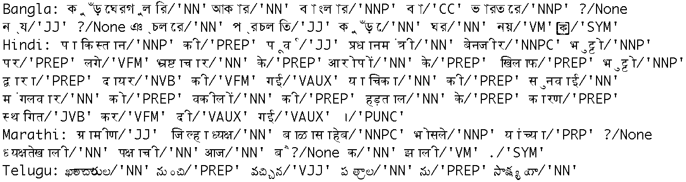
Figure 3.1: POS-Tagged Data from Four Indian Languages

If the corpus is also segmented into sentences, it will have a tagged_sents() method that returns a list of tagged sentences. This will be useful when we come to training automatic taggers, as they typically function on a sentence at a time.

3.2.2   Nouns and Verbs

Linguists recognize several major categories of words in English, such as nouns, verbs, adjectives and determiners. In this section we will discuss the most important categories, namely nouns and verbs.

Nouns generally refer to people, places, things, or concepts, e.g.: woman, Scotland, book, intelligence. Nouns can appear after determiners and adjectives, and can be the subject or object of the verb, as shown in Table 3.2.

Table 3.2:

Syntactic Patterns involving some Nouns

Nouns can be classified as common nouns and proper nouns. Proper nouns identify particular individuals or entities, e.g. Moses and Scotland. Common nouns are all the rest. Another distinction exists between count nouns and mass nouns. Count nouns are thought of as distinct entities that can be counted, such as pig (e.g. one pig, two pigs, many pigs). They cannot occur with the word much (i.e. *much pigs). Mass nouns, on the other hand, are not thought of as distinct entities (e.g. sand). They cannot be pluralized, and do not occur with numbers (e.g. *two sands, *many sands). However, they can occur with much (i.e. much sand).

Verbs are words that describe events and actions, e.g. fall, eat in Table 3.3. In the context of a sentence, verbs express a relation involving the referents of one or more noun phrases.

Table 3.3:

Syntactic Patterns involving some Verbs

Verbs can be classified according to the number of arguments (usually noun phrases) that they require. The word fall is intransitive, requiring exactly one argument (the entity that falls). The word eat is transitive, requiring two arguments (the eater and the eaten). Other verbs are more complex; for instance put requires three arguments, the agent doing the putting, the entity being put somewhere, and a location. We will return to this topic when we come to look at grammars and parsing (see Chapter 7).

In the Brown Corpus, verbs have a range of possible tags, e.g.: give/VB (present), gives/VBZ (present, 3ps), giving/VBG (present continuous; gerund) gave/VBD (simple past), and given/VBN (past participle). We will discuss these tags in more detail in a later section.

3.2.3   Nouns and Verbs in Tagged Corpora

Now that we are able to access tagged corpora, we can write simple programs to garner statistics about the tags. In this section we will focus on the nouns and verbs.

What are the 10 most common verbs? We can write a program to find all words tagged with VB, VBZ, VBG, VBD or VBN.

>>> fd = nltk.FreqDist()
>>> for (wd, tg) in nltk.corpus.brown.tagged_words(categories='a'):
...     if tg[:2] == 'VB':
...         fd.inc(wd + "/" + tg)
>>> fd.sorted()[:20]
['said/VBD', 'get/VB', 'made/VBN', 'United/VBN-TL', 'take/VB',
 'took/VBD', 'told/VBD', 'made/VBD', 'make/VB', 'got/VBD',
 'came/VBD', 'go/VB', 'see/VB', 'went/VBD', 'given/VBN',
 'expected/VBN', 'began/VBD', 'give/VB', 'taken/VBN', 'play/VB']

Let's study nouns, and find the most frequent nouns of each noun part-of-speech type. The program in Listing 3.2 finds all tags starting with NN, and provides a few example words for each one. Observe that there are many noun tags; the most important of these have $ for possessive nouns, S for plural nouns (since plural nouns typically end in s), P for proper nouns.

def findtags(tag_prefix, tagged_text):
    cfd = nltk.ConditionalFreqDist()
    for (wd, tg) in tagged_text:
        if tg.startswith(tag_prefix):
            cfd[tg].inc(wd)
    tagdict = {}
    for tg in cfd.conditions():
        tagdict[tg] = cfd[tg].sorted()[:5]
    return tagdict

>>> tagdict = findtags('NN', nltk.corpus.brown.tagged_words(categories='a'))
>>> for tg in sorted(tagdict):
...     print tg, tagdict[tg]
NN ['year', 'time', 'state', 'week', 'man']
NN$ ["year's", "world's", "state's", "nation's", "company's"]
NN$-HL ["Golf's", "Navy's"]
NN$-TL ["President's", "University's", "League's", "Gallery's", "Army's"]
NN-HL ['cut', 'Salary', 'condition', 'Question', 'business']
NN-NC ['eva', 'ova', 'aya']
NN-TL ['President', 'House', 'State', 'University', 'City']
NN-TL-HL ['Fort', 'City', 'Commissioner', 'Grove', 'House']
NNS ['years', 'members', 'people', 'sales', 'men']
NNS$ ["children's", "women's", "men's", "janitors'", "taxpayers'"]
NNS$-HL ["Dealers'", "Idols'"]
NNS$-TL ["Women's", "States'", "Giants'", "Officers'", "Bombers'"]
NNS-HL ['years', 'idols', 'Creations', 'thanks', 'centers']
NNS-TL ['States', 'Nations', 'Masters', 'Rules', 'Communists']
NNS-TL-HL ['Nations']

Some tags contain a plus sign; these are compound tags, and are assigned to words that contain two parts normally treated separately. Some tags contain a minus sign; this indicates disjunction.

3.2.4   The Default Tagger

The simplest possible tagger assigns the same tag to each token. This may seem to be a rather banal step, but it establishes an important baseline for tagger performance. In order to get the best result, we tag each word with the most likely word. (This kind of tagger is known as a majority class classifier). What then, is the most frequent tag? We can find out using a simple program:

>>> fd = nltk.FreqDist()
>>> for (wd, tg) in nltk.corpus.brown.tagged_words(categories='a'):
...     fd.inc(tg)
>>> fd.max()
'NN'

>>> tokens = 'John saw 3 polar bears .'.split()
>>> default_tagger = nltk.DefaultTagger('NN')
>>> default_tagger.tag(tokens)
[('John', 'NN'), ('saw', 'NN'), ('3', 'NN'), ('polar', 'NN'),
('bears', 'NN'), ('.', 'NN')]

>>> nltk.tag.accuracy(default_tagger, nltk.corpus.brown.tagged_sents(categories='a'))
0.13089484257215028

English verbs can also be morphologically complex. For instance, the present participle of a verb ends in -ing, and expresses the idea of ongoing, incomplete action (e.g. falling, eating). The -ing suffix also appears on nouns derived from verbs, e.g. the falling of the leaves (this is known as the gerund). In the Brown corpus, these are tagged VBG.

The past participle of a verb often ends in -ed, and expresses the idea of a completed action (e.g. walked, cried). These are tagged VBD.

Common tag sets often capture some morpho-syntactic information; that is, information about the kind of morphological markings that words receive by virtue of their syntactic role. Consider, for example, the selection of distinct grammatical forms of the word go illustrated in the following sentences:

We can easily imagine a tag set in which the four distinct grammatical forms just discussed were all tagged as VB. Although this would be adequate for some purposes, a more fine-grained tag set will provide useful information about these forms that can be of value to other processors that try to detect syntactic patterns from tag sequences. As we noted at the beginning of this chapter, the Brown tag set does in fact capture these distinctions, as summarized in Table 3.4.

Table 3.4:

Some morphosyntactic distinctions in the Brown tag set

In addition to this set of verb tags, the various forms of the verb to be have special tags: be/BE, being/BEG, am/BEM, been/BEN and was/BEDZ. All told, this fine-grained tagging of verbs means that an automatic tagger that uses this tag set is in effect carrying out a limited amount of morphological analysis.

Most part-of-speech tag sets make use of the same basic categories, such as noun, verb, adjective, and preposition. However, tag sets differ both in how finely they divide words into categories, and in how they define their categories. For example, is might be tagged simply as a verb in one tag set; but as a distinct form of the lexeme BE in another tag set (as in the Brown Corpus). This variation in tag sets is unavoidable, since part-of-speech tags are used in different ways for different tasks. In other words, there is no one 'right way' to assign tags, only more or less useful ways depending on one's goals. More details about the Brown corpus tag set can be found in the Appendix at the end of this chapter.

3.3.2   The Regular Expression Tagger

The regular expression tagger assigns tags to tokens on the basis of matching patterns. For instance, we might guess that any word ending in ed is the past participle of a verb, and any word ending with 's is a possessive noun. We can express these as a list of regular expressions:

>>> patterns = [
...     (r'.*ing$', 'VBG'),               # gerunds
...     (r'.*ed$', 'VBD'),                # simple past
...     (r'.*es$', 'VBZ'),                # 3rd singular present
...     (r'.*ould$', 'MD'),               # modals
...     (r'.*\'s$', 'NN$'),               # possessive nouns
...     (r'.*s$', 'NNS'),                 # plural nouns
...     (r'^-?[0-9]+(.[0-9]+)?$', 'CD'),  # cardinal numbers
...     (r'.*', 'NN')                     # nouns (default)
... ]

Note that these are processed in order, and the first one that matches is applied.

Now we can set up a tagger and use it to tag some text.

>>> regexp_tagger = nltk.RegexpTagger(patterns)
>>> regexp_tagger.tag(nltk.corpus.brown.sents(categories='a')[3])
[('``', 'NN'), ('Only', 'NN'), ('a', 'NN'), ('relative', 'NN'),
('handful', 'NN'), ('of', 'NN'), ('such', 'NN'), ('reports', 'NNS'),
('was', 'NNS'), ('received', 'VBD'), ("''", 'NN'), (',', 'NN'),
('the', 'NN'), ('jury', 'NN'), ('said', 'NN'), (',', 'NN'), ('``', 'NN'),
('considering', 'VBG'), ('the', 'NN'), ('widespread', 'NN'), ..., ('.', 'NN')]

How well does this do?

>>> nltk.tag.accuracy(regexp_tagger, nltk.corpus.brown.tagged_sents(categories='a'))
0.20326391789486245

The regular expression is a catch-all that tags everything as a noun. This is equivalent to the default tagger (only much less efficient). Instead of re-specifying this as part of the regular expression tagger, is there a way to combine this tagger with the default tagger? We will see how to do this later, under the heading of backoff taggers.

3.3.3   Exercises

1. ☼ Search the web for "spoof newspaper headlines", to find such gems as: British Left Waffles on Falkland Islands, and Juvenile Court to Try Shooting Defendant. Manually tag these headlines to see if knowledge of the part-of-speech tags removes the ambiguity.
2. ☼ Satisfy yourself that there are restrictions on the distribution of go and went, in the sense that they cannot be freely interchanged in the kinds of contexts illustrated in (1d).
3. ◑ Write code to search the Brown Corpus for particular words and phrases according to tags, to answer the following questions:
   1. Produce an alphabetically sorted list of the distinct words tagged as MD.
   2. Identify words that can be plural nouns or third person singular verbs (e.g. deals, flies).
   3. Identify three-word prepositional phrases of the form IN + DET + NN (eg. in the lab).
   4. What is the ratio of masculine to feminine pronouns?
4. ◑ In the introduction we saw a table involving frequency counts for the verbs adore, love, like, prefer and preceding qualifiers such as really. Investigate the full range of qualifiers (Brown tag QL) that appear before these four verbs.
5. ◑ We defined the regexp_tagger that can be used as a fall-back tagger for unknown words. This tagger only checks for cardinal numbers. By testing for particular prefix or suffix strings, it should be possible to guess other tags. For example, we could tag any word that ends with -s as a plural noun. Define a regular expression tagger (using nltk.RegexpTagger) that tests for at least five other patterns in the spelling of words. (Use inline documentation to explain the rules.)
6. ◑ Consider the regular expression tagger developed in the exercises in the previous section. Evaluate the tagger using nltk.tag.accuracy(), and try to come up with ways to improve its performance. Discuss your findings. How does objective evaluation help in the development process?
7. ★ There are 264 distinct words in the Brown Corpus having exactly three possible tags.
   1. Print a table with the integers 1..10 in one column, and the number of distinct words in the corpus having 1..10 distinct tags.
   2. For the word with the greatest number of distinct tags, print out sentences from the corpus containing the word, one for each possible tag.
8. ★ Write a program to classify contexts involving the word must according to the tag of the following word. Can this be used to discriminate between the epistemic and deontic uses of must?

3.4.1   The Lookup Tagger

A lot of high-frequency words do not have the NN tag. Let's find some of these words and their tags. The following code takes a list of sentences and counts up the words, and prints the 100 most frequent words:

>>> fd = nltk.FreqDist(nltk.corpus.brown.words(categories='a'))
>>> most_freq_words = fd.sorted()[:100]
>>> most_freq_words
['the', ',', '.', 'of', 'and', 'to', 'a', 'in', 'for', 'The', 'that', '``',
'is', 'was', "''", 'on', 'at', 'with', 'be', 'by', 'as', 'he', 'said', 'his',
'will', 'it', 'from', 'are', ';', 'has', 'an', '--', 'had', 'who', 'have',
'not', 'Mrs.', 'were', 'this', 'would', 'which', 'their', 'been', 'they', 'He',
'one', 'I', 'its', 'but', 'or', 'more', ')', 'Mr.', 'up', '(', 'all', 'last',
'out', 'two', ':', 'other', 'new', 'first', 'year', 'than', 'A', 'about', 'there',
'when', 'home', 'after', 'In', 'also', 'over', 'It', 'into', 'no', 'But', 'made',
'her', 'only', 'years', 'time', 'three', 'them', 'some', 'can', 'New', 'him',
'state', '?', 'any', 'President', 'could', 'before', 'week', 'under', 'against',
'we', 'now']

Next, let's inspect the tags that these words have. First we will do this in the most obvious (but highly inefficient) way:

>>> [(w,t) for (w,t) in nltk.corpus.brown.tagged_words(categories='a')
...        if w in most_freq_words]
[('The', 'AT'), ('said', 'VBD'), ('an', 'AT'), ('of', 'IN'),
('``', '``'), ('no', 'AT'), ("''", "''"), ('that', 'CS'),
('any', 'DTI'), ('.', '.'), ..., ("''", "''")]

A much better approach is to set up a dictionary that maps each of the 100 most frequent words to its most likely tag. We can do this by setting up a frequency distribution cfd over the tagged words, i.e. the frequency of the different tags that occur with each word.

>>> cfd = nltk.ConditionalFreqDist(nltk.corpus.brown.tagged_words(categories='a'))

Now for any word that appears in this section of the corpus, we can determine its most likely tag:

>>> likely_tags = dict((word, cfd[word].max()) for word in most_freq_words)
>>> likely_tags['The']
'AT'

Finally, we can create and evaluate a simple tagger that assigns tags to words based on this table:

>>> baseline_tagger = nltk.UnigramTagger(model=likely_tags)
>>> nltk.tag.accuracy(baseline_tagger, nltk.corpus.brown.tagged_sents(categories='a'))
0.45578495136941344

This is surprisingly good; just knowing the tags for the 100 most frequent words enables us to tag nearly half of all words correctly! Let's see what it does on some untagged input text:

>>> baseline_tagger.tag(nltk.corpus.brown.sents(categories='a')[3])
[('``', '``'), ('Only', None), ('a', 'AT'), ('relative', None),
('handful', None), ('of', 'IN'), ('such', None), ('reports', None),
('was', 'BEDZ'), ('received', None), ("''", "''"), (',', ','),
('the', 'AT'), ('jury', None), ('said', 'VBD'), (',', ','),
('``', '``'), ('considering', None), ('the', 'AT'), ('widespread', None),
('interest', None), ('in', 'IN'), ('the', 'AT'), ('election', None),
(',', ','), ('the', 'AT'), ('number', None), ('of', 'IN'),
('voters', None), ('and', 'CC'), ('the', 'AT'), ('size', None),
('of', 'IN'), ('this', 'DT'), ('city', None), ("''", "''"), ('.', '.')]

Notice that a lot of these words have been assigned a tag of None. That is because they were not among the 100 most frequent words. In these cases we would like to assign the default tag of NN, a process known as backoff.

3.4.2   Backoff

How do we combine these taggers? We want to use the lookup table first, and if it is unable to assign a tag, then use the default tagger. We do this by specifying the default tagger as an argument to the lookup tagger. The lookup tagger will call the default tagger just in case it can't assign a tag itself.

>>> baseline_tagger = nltk.UnigramTagger(model=likely_tags, backoff=nltk.DefaultTagger('NN'))
>>> nltk.tag.accuracy(baseline_tagger, nltk.corpus.brown.tagged_sents(categories='a'))
0.58177695566561249

We will return to this technique in the context of a broader discussion on combining taggers in Section 3.5.6.

3.4.3   Choosing a Good Baseline

We can put all this together to write a simple (but somewhat inefficient) program to create and evaluate lookup taggers having a range of sizes, as shown in Listing 3.3. We include a backoff tagger that tags everything as a noun. A consequence of using this backoff tagger is that the lookup tagger only has to store word/tag pairs for words other than nouns.

def performance(cfd, wordlist):
    lt = dict((word, cfd[word].max()) for word in wordlist)
    baseline_tagger = nltk.UnigramTagger(model=lt, backoff=nltk.DefaultTagger('NN'))
    return nltk.tag.accuracy(baseline_tagger, nltk.corpus.brown.tagged_sents(categories='a'))

def display():
    import pylab
    words_by_freq = nltk.FreqDist(nltk.corpus.brown.words(categories='a')).sorted()
    cfd = nltk.ConditionalFreqDist(nltk.corpus.brown.tagged_words(categories='a'))
    sizes = 2 ** pylab.arange(15)
    perfs = [performance(cfd, words_by_freq[:size]) for size in sizes]
    pylab.plot(sizes, perfs, '-bo')
    pylab.title('Lookup Tagger Performance with Varying Model Size')
    pylab.xlabel('Model Size')
    pylab.ylabel('Performance')
    pylab.show()

>>> display()                                  

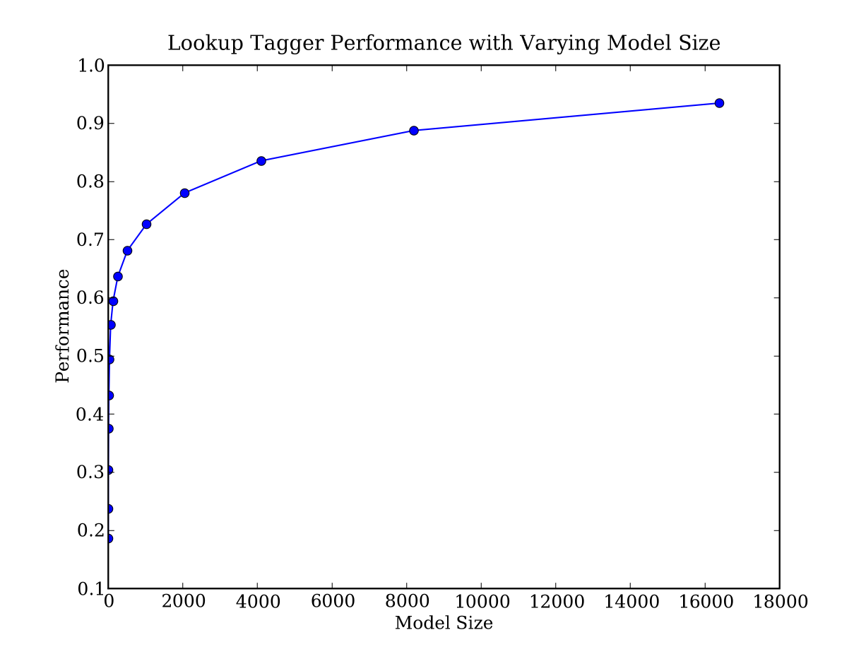
Figure 3.2: Lookup Tagger

Observe that performance initially increases rapidly as the model size grows, eventually reaching a plateau, when large increases in model size yield little improvement in performance. (This example used the pylab plotting package; we will return to this later in Section 5.3.4).

3.4.4   Exercises

1. ◑ Explore the following issues that arise in connection with the lookup tagger:
   1. What happens to the tagger performance for the various model sizes when a backoff tagger is omitted?
   2. Consider the curve in Figure 3.2; suggest a good size for a lookup tagger that balances memory and performance. Can you come up with scenarios where it would be preferable to minimize memory usage, or to maximize performance with no regard for memory usage?
2. ◑ What is the upper limit of performance for a lookup tagger, assuming no limit to the size of its table? (Hint: write a program to work out what percentage of tokens of a word are assigned the most likely tag for that word, on average.)

3.5.1   More English Word Classes

Two other important word classes are adjectives and adverbs. Adjectives describe nouns, and can be used as modifiers (e.g. large in the large pizza), or in predicates (e.g. the pizza is large). English adjectives can be morphologically complex (e.g. fall_V+ing in the falling stocks). Adverbs modify verbs to specify the time, manner, place or direction of the event described by the verb (e.g. quickly in the stocks fell quickly). Adverbs may also modify adjectives (e.g. really in Mary's teacher was really nice).

English has several categories of closed class words in addition to prepositions, such as articles (also often called determiners) (e.g., the, a), modals (e.g., should, may), and personal pronouns (e.g., she, they). Each dictionary and grammar classifies these words differently.

Part-of-speech tags are closely related to the notion of word class used in syntax. The assumption in linguistics is that every distinct word type will be listed in a lexicon (or dictionary), with information about its pronunciation, syntactic properties and meaning. A key component of the word's properties will be its class. When we carry out a syntactic analysis of an example like fruit flies like a banana, we will look up each word in the lexicon, determine its word class, and then group it into a hierarchy of phrases, as illustrated in the following parse tree.

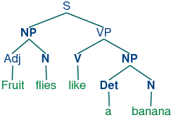
Syntactic analysis will be dealt with in more detail in Part II. For now, we simply want to make the connection between the labels used in syntactic parse trees and part-of-speech tags. Table 3.5 shows the correspondence:

Table 3.5:

Word Class Labels and Brown Corpus Tags

3.5.2   Some Diagnostics

Now that we have examined word classes in detail, we turn to a more basic question: how do we decide what category a word belongs to in the first place? In general, linguists use three criteria: morphological (or formal); syntactic (or distributional); semantic (or notional). A morphological criterion is one that looks at the internal structure of a word. For example, -ness is a suffix that combines with an adjective to produce a noun. Examples are happy → happiness, ill → illness. So if we encounter a word that ends in -ness, this is very likely to be a noun.

A syntactic criterion refers to the contexts in which a word can occur. For example, assume that we have already determined the category of nouns. Then we might say that a syntactic criterion for an adjective in English is that it can occur immediately before a noun, or immediately following the words be or very. According to these tests, near should be categorized as an adjective:

A familiar example of a semantic criterion is that a noun is "the name of a person, place or thing". Within modern linguistics, semantic criteria for word classes are treated with suspicion, mainly because they are hard to formalize. Nevertheless, semantic criteria underpin many of our intuitions about word classes, and enable us to make a good guess about the categorization of words in languages that we are unfamiliar with. For example, if we all we know about the Dutch verjaardag is that it means the same as the English word birthday, then we can guess that verjaardag is a noun in Dutch. However, some care is needed: although we might translate zij is vandaag jarig as it's her birthday today, the word jarig is in fact an adjective in Dutch, and has no exact equivalent in English!

All languages acquire new lexical items. A list of words recently added to the Oxford Dictionary of English includes cyberslacker, fatoush, blamestorm, SARS, cantopop, bupkis, noughties, muggle, and robata. Notice that all these new words are nouns, and this is reflected in calling nouns an open class. By contrast, prepositions are regarded as a closed class. That is, there is a limited set of words belonging to the class (e.g., above, along, at, below, beside, between, during, for, from, in, near, on, outside, over, past, through, towards, under, up, with), and membership of the set only changes very gradually over time.

Unigram taggers are based on a simple statistical algorithm: for each token, assign the tag that is most likely for that particular token. For example, it will assign the tag JJ to any occurrence of the word frequent, since frequent is used as an adjective (e.g. a frequent word) more often than it is used as a verb (e.g. I frequent this cafe). A unigram tagger behaves just like a lookup tagger (Section 3.4.1), except there is a more convenient technique for setting it up, called training. In the following code sample, we initialize and train a unigram tagger (line ), use it to tag a sentence, then finally compute the tagger's overall accuracy:

>>> brown_a = nltk.corpus.brown.tagged_sents(categories='a')
>>> unigram_tagger = nltk.UnigramTagger(brown_a)               
>>> sent = nltk.corpus.brown.sents(categories='a')[2007]
>>> unigram_tagger.tag(sent)
[('Various', None), ('of', 'IN'), ('the', 'AT'), ('apartments', 'NNS'), ('are', 'BER'),
('of', 'IN'), ('the', 'AT'), ('terrace', 'NN'), ('type', 'NN'), (',', ','),
('being', 'BEG'), ('on', 'IN'), ('the', 'AT'), ('ground', 'NN'), ('floor', 'NN'),
('so', 'QL'), ('that', 'CS'), ('entrance', 'NN'), ('is', 'BEZ'), ('direct', 'JJ'), ('.', '.')]
>>> nltk.tag.accuracy(unigram_tagger, brown_a)
0.8550331165343994

3.5.4   Affix Taggers

Affix taggers are like unigram taggers, except they are trained on word prefixes or suffixes of a specified length. (NB. Here we use prefix and suffix in the string sense, not the morphological sense.) For example, the following tagger will consider suffixes of length 3 (e.g. -ize, -ion), for words having at least 5 characters.

>>> affix_tagger = nltk.AffixTagger(brown_a, affix_length=-2, min_stem_length=3)
>>> affix_tagger.tag(sent)
[('Various', 'JJ'), ('of', None), ('the', None), ('apartments', 'NNS'), ('are', None),
('of', None), ('the', None), ('terrace', 'NN'), ('type', None), (',', None),
('being', 'VBG'), ('on', None), ('the', None), ('ground', 'NN'), ('floor', 'NN'),
('so', None), ('that', None), ('entrance', 'NN'), ('is', None), ('direct', 'NN'),
('.', None)]

3.5.5   N-Gram Taggers

When we perform a language processing task based on unigrams, we are using one item of context. In the case of tagging, we only consider the current token, in isolation from any larger context. Given such a model, the best we can do is tag each word with its a priori most likely tag. This means we would tag a word such as wind with the same tag, regardless of whether it appears in the context the wind or to wind.

An n-gram tagger is a generalization of a unigram tagger whose context is the current word together with the part-of-speech tags of the n-1 preceding tokens, as shown in Figure 3.3. The tag to be chosen, t_n, is circled, and the context is shaded in grey. In the example of an n-gram tagger shown in Figure 3.3, we have n=3; that is, we consider the tags of the two preceding words in addition to the current word. An n-gram tagger picks the tag that is most likely in the given context.

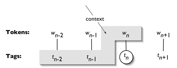
Figure 3.3: Tagger Context

The NgramTagger class uses a tagged training corpus to determine which part-of-speech tag is most likely for each context. Here we see a special case of an n-gram tagger, namely a bigram tagger. First we train it, then use it to tag untagged sentences:

>>> bigram_tagger = nltk.BigramTagger(brown_a, cutoff=0)
>>> bigram_tagger.tag(sent)
[('Various', 'JJ'), ('of', 'IN'), ('the', 'AT'), ('apartments', 'NNS'), ('are', 'BER'),
('of', 'IN'), ('the', 'AT'), ('terrace', 'NN'), ('type', 'NN'), (',', ','),
('being', 'BEG'), ('on', 'IN'), ('the', 'AT'), ('ground', 'NN'), ('floor', 'NN'),
('so', 'CS'), ('that', 'CS'), ('entrance', 'NN'), ('is', 'BEZ'), ('direct', 'JJ'),
('.', '.')]

As with the other taggers, n-gram taggers assign the tag None to any token whose context was not seen during training.

As n gets larger, the specificity of the contexts increases, as does the chance that the data we wish to tag contains contexts that were not present in the training data. This is known as the sparse data problem, and is quite pervasive in NLP. Thus, there is a trade-off between the accuracy and the coverage of our results (and this is related to the precision/recall trade-off in information retrieval).

Our approach to tagging unknown words still uses backoff to a regular-expression tagger or a default tagger. These are unable to make use of context. Thus, if our tagger encountered the word blog, not seen during training, it would assign it a tag regardless of whether this word appeared in the context the blog or to blog. How can we do better with these unknown words, or out-of-vocabulary items?

1. ☼ Train a unigram tagger and run it on some new text. Observe that some words are not assigned a tag. Why not?
2. ☼ Train an affix tagger AffixTagger() and run it on some new text. Experiment with different settings for the affix length and the minimum word length. Can you find a setting that seems to perform better than the one described above? Discuss your findings.
3. ☼ Train a bigram tagger with no backoff tagger, and run it on some of the training data. Next, run it on some new data. What happens to the performance of the tagger? Why?
4. ◑ Write a program that calls AffixTagger() repeatedly, using different settings for the affix length and the minimum word length. What parameter values give the best overall performance? Why do you think this is the case?
5. ◑ How serious is the sparse data problem? Investigate the performance of n-gram taggers as n increases from 1 to 6. Tabulate the accuracy score. Estimate the training data required for these taggers, assuming a vocabulary size of 10⁵ and a tagset size of 10².
6. ◑ Obtain some tagged data for another language, and train and evaluate a variety of taggers on it. If the language is morphologically complex, or if there are any orthographic clues (e.g. capitalization) to word classes, consider developing a regular expression tagger for it (ordered after the unigram tagger, and before the default tagger). How does the accuracy of your tagger(s) compare with the same taggers run on English data? Discuss any issues you encounter in applying these methods to the language.
7. ★ Create a default tagger and various unigram and n-gram taggers, incorporating backoff, and train them on part of the Brown corpus.
   1. Create three different combinations of the taggers. Test the accuracy of each combined tagger. Which combination works best?
   2. Try varying the size of the training corpus. How does it affect your results?
8. ★ Our approach for tagging an unknown word has been to consider the letters of the word (using RegexpTagger() and AffixTagger()), or to ignore the word altogether and tag it as a noun (using nltk.DefaultTagger()). These methods will not do well for texts having new words that are not nouns. Consider the sentence I like to blog on Kim's blog. If blog is a new word, then looking at the previous tag (TO vs NP$) would probably be helpful. I.e. we need a default tagger that is sensitive to the preceding tag.
   1. Create a new kind of unigram tagger that looks at the tag of the previous word, and ignores the current word. (The best way to do this is to modify the source code for UnigramTagger(), which presumes knowledge of Python classes discussed in Section 9.)
   2. Add this tagger to the sequence of backoff taggers (including ordinary trigram and bigram taggers that look at words), right before the usual default tagger.
   3. Evaluate the contribution of this new unigram tagger.
9. ★ Write code to preprocess tagged training data, replacing all but the most frequent n words with the special word UNK. Train an n-gram backoff tagger on this data, then use it to tag some new text. Note that you will have to preprocess the text to replace unknown words with UNK, and post-process the tagged output to replace the UNK words with the words from the original input.

3.8.1   Acknowledgments