OpenCV  3.0.0-dev
Open Source Computer Vision
Histogram Comparison

Goal

In this tutorial you will learn how to:

Theory

Code

#include <iostream>
#include <stdio.h>
using namespace std;
using namespace cv;
int main( int argc, char** argv )
{
Mat src_base, hsv_base;
Mat src_test1, hsv_test1;
Mat src_test2, hsv_test2;
Mat hsv_half_down;
if( argc < 4 )
{
printf("** Error. Usage: ./compareHist_Demo <image_settings0> <image_setting1> <image_settings2>\n");
return -1;
}
src_base = imread( argv[1], 1 );
src_test1 = imread( argv[2], 1 );
src_test2 = imread( argv[3], 1 );
cvtColor( src_base, hsv_base, COLOR_BGR2HSV );
cvtColor( src_test1, hsv_test1, COLOR_BGR2HSV );
cvtColor( src_test2, hsv_test2, COLOR_BGR2HSV );
hsv_half_down = hsv_base( Range( hsv_base.rows/2, hsv_base.rows - 1 ), Range( 0, hsv_base.cols - 1 ) );
int h_bins = 50; int s_bins = 60;
int histSize[] = { h_bins, s_bins };
// hue varies from 0 to 179, saturation from 0 to 255
float h_ranges[] = { 0, 180 };
float s_ranges[] = { 0, 256 };
const float* ranges[] = { h_ranges, s_ranges };
// Use the o-th and 1-st channels
int channels[] = { 0, 1 };
MatND hist_base;
MatND hist_half_down;
MatND hist_test1;
MatND hist_test2;
calcHist( &hsv_base, 1, channels, Mat(), hist_base, 2, histSize, ranges, true, false );
normalize( hist_base, hist_base, 0, 1, NORM_MINMAX, -1, Mat() );
calcHist( &hsv_half_down, 1, channels, Mat(), hist_half_down, 2, histSize, ranges, true, false );
normalize( hist_half_down, hist_half_down, 0, 1, NORM_MINMAX, -1, Mat() );
calcHist( &hsv_test1, 1, channels, Mat(), hist_test1, 2, histSize, ranges, true, false );
normalize( hist_test1, hist_test1, 0, 1, NORM_MINMAX, -1, Mat() );
calcHist( &hsv_test2, 1, channels, Mat(), hist_test2, 2, histSize, ranges, true, false );
normalize( hist_test2, hist_test2, 0, 1, NORM_MINMAX, -1, Mat() );
for( int i = 0; i < 4; i++ )
{
int compare_method = i;
double base_base = compareHist( hist_base, hist_base, compare_method );
double base_half = compareHist( hist_base, hist_half_down, compare_method );
double base_test1 = compareHist( hist_base, hist_test1, compare_method );
double base_test2 = compareHist( hist_base, hist_test2, compare_method );
printf( " Method [%d] Perfect, Base-Half, Base-Test(1), Base-Test(2) : %f, %f, %f, %f \n", i, base_base, base_half , base_test1, base_test2 );
}
printf( "Done \n" );
return 0;
}

Explanation

  1. Declare variables such as the matrices to store the base image and the two other images to compare ( BGR and HSV )
    Mat src_base, hsv_base;
    Mat src_test1, hsv_test1;
    Mat src_test2, hsv_test2;
    Mat hsv_half_down;
  2. Load the base image (src_base) and the other two test images:
    if( argc < 4 )
    { printf("** Error. Usage: ./compareHist_Demo <image_settings0> <image_setting1> <image_settings2>\n");
    return -1;
    }
    src_base = imread( argv[1], 1 );
    src_test1 = imread( argv[2], 1 );
    src_test2 = imread( argv[3], 1 );
  3. Convert them to HSV format:
    cvtColor( src_base, hsv_base, COLOR_BGR2HSV );
    cvtColor( src_test1, hsv_test1, COLOR_BGR2HSV );
    cvtColor( src_test2, hsv_test2, COLOR_BGR2HSV );
  4. Also, create an image of half the base image (in HSV format):
    hsv_half_down = hsv_base( Range( hsv_base.rows/2, hsv_base.rows - 1 ), Range( 0, hsv_base.cols - 1 ) );
  5. Initialize the arguments to calculate the histograms (bins, ranges and channels H and S ).
    int h_bins = 50; int s_bins = 60;
    int histSize[] = { h_bins, s_bins };
    float h_ranges[] = { 0, 180 };
    float s_ranges[] = { 0, 256 };
    const float* ranges[] = { h_ranges, s_ranges };
    int channels[] = { 0, 1 };
  6. Create the MatND objects to store the histograms:
    MatND hist_base;
    MatND hist_half_down;
    MatND hist_test1;
    MatND hist_test2;
  7. Calculate the Histograms for the base image, the 2 test images and the half-down base image:
    calcHist( &hsv_base, 1, channels, Mat(), hist_base, 2, histSize, ranges, true, false );
    normalize( hist_base, hist_base, 0, 1, NORM_MINMAX, -1, Mat() );
    calcHist( &hsv_half_down, 1, channels, Mat(), hist_half_down, 2, histSize, ranges, true, false );
    normalize( hist_half_down, hist_half_down, 0, 1, NORM_MINMAX, -1, Mat() );
    calcHist( &hsv_test1, 1, channels, Mat(), hist_test1, 2, histSize, ranges, true, false );
    normalize( hist_test1, hist_test1, 0, 1, NORM_MINMAX, -1, Mat() );
    calcHist( &hsv_test2, 1, channels, Mat(), hist_test2, 2, histSize, ranges, true, false );
    normalize( hist_test2, hist_test2, 0, 1, NORM_MINMAX, -1, Mat() );
  8. Apply sequentially the 4 comparison methods between the histogram of the base image (hist_base) and the other histograms:
    for( int i = 0; i < 4; i++ )
    { int compare_method = i;
    double base_base = compareHist( hist_base, hist_base, compare_method );
    double base_half = compareHist( hist_base, hist_half_down, compare_method );
    double base_test1 = compareHist( hist_base, hist_test1, compare_method );
    double base_test2 = compareHist( hist_base, hist_test2, compare_method );
    printf( " Method [%d] Perfect, Base-Half, Base-Test(1), Base-Test(2) : %f, %f, %f, %f \n", i, base_base, base_half , base_test1, base_test2 );
    }

Results

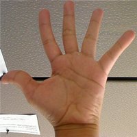
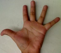
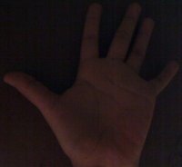
  1. We use as input the following images:
    Histogram_Comparison_Source_0.jpg
    Base_0
    Histogram_Comparison_Source_1.jpg
    Test_1
    Histogram_Comparison_Source_2.jpg
    Test_2
    where the first one is the base (to be compared to the others), the other 2 are the test images. We will also compare the first image with respect to itself and with respect of half the base image.
  2. We should expect a perfect match when we compare the base image histogram with itself. Also, compared with the histogram of half the base image, it should present a high match since both are from the same source. For the other two test images, we can observe that they have very different lighting conditions, so the matching should not be very good:
  3. Here the numeric results:
    *Method* Base - Base Base - Half Base - Test 1 Base - Test 2
    *Correlation* 1.000000 0.930766 0.182073 0.120447
    *Chi-square* 0.000000 4.940466 21.184536 49.273437
    *Intersection* 24.391548 14.959809 3.889029 5.775088
    *Bhattacharyya* 0.000000 0.222609 0.646576 0.801869
    For the Correlation and Intersection methods, the higher the metric, the more accurate the match. As we can see, the match base-base is the highest of all as expected. Also we can observe that the match base-half is the second best match (as we predicted). For the other two metrics, the less the result, the better the match. We can observe that the matches between the test 1 and test 2 with respect to the base are worse, which again, was expected.