App Trace Roll: Users Guide: 
| ||
|---|---|---|
| Prev | Chapter 3. Using the App Trace Roll | Next |
If you wish analyze the data, follow the procedure in this section. If not and you would like to upload your trace files to SDSC, skip to the next section Uploading Trace Files to SDSC.
To download all the traces from all the compute nodes, execute:
# make -f /opt/app-trace/collect/Makefile local |
The above command will store all traces in /state/partition1/traces.
 | Collecting the trace files stops the trace function on each node. If you wish to trace more applications after collecting the trace data, you'll need to reexecute a command like:
|
Then to build plots for specific executables, first go to the directory that has the recently downloaded traces:
# cd /state/partition1/traces |
Then, determine the directory that was created by the above collection. Below is an example listing:
# ls | sort 1132195141.948881000 1132195260.675707000 1132195264.174861000 |
The last directory is the most recently created one. Now, let's build some I/O trace graphs from the recently created collection:
# cd 1132195264.174861000 # make -f /opt/app-trace/analyze/bin/Makefile PROGRAMS=iozone,dd |
The above will build graphs for every instance of the programs iozone and dd that were running on all the compute nodes over the trace interval.
The resulting graphs are put under /var/www/html/rocks-app-trace/analyze/. This directory contains a subdirecties that are labeled for each node that trace data was collected from.
Point your web browser at http://10.1.1.1/rocks-app-trace/analyze and navigate into the node directory names. In the example above, there are the files:
trace-disk-iozone-8974-read-0.plot.png trace-disk-iozone-8974-read-1.plot.png trace-disk-iozone-8974-read-2.plot.png trace-disk-iozone-8974-read-3.plot.png trace-disk-iozone-8974-read-4.plot.png trace-disk-iozone-8974-read,write,seek.plot.png trace-disk-iozone-8974-seek-0.plot.png trace-disk-iozone-8974-seek-1.plot.png trace-disk-iozone-8974-seek-2.plot.png trace-disk-iozone-8974-seek-3.plot.png trace-disk-iozone-8974-write-0.plot.png trace-disk-iozone-8974-write-1.plot.png trace-disk-iozone-8974-write-2.plot.png trace-disk-iozone-8974-write-3.plot.png |
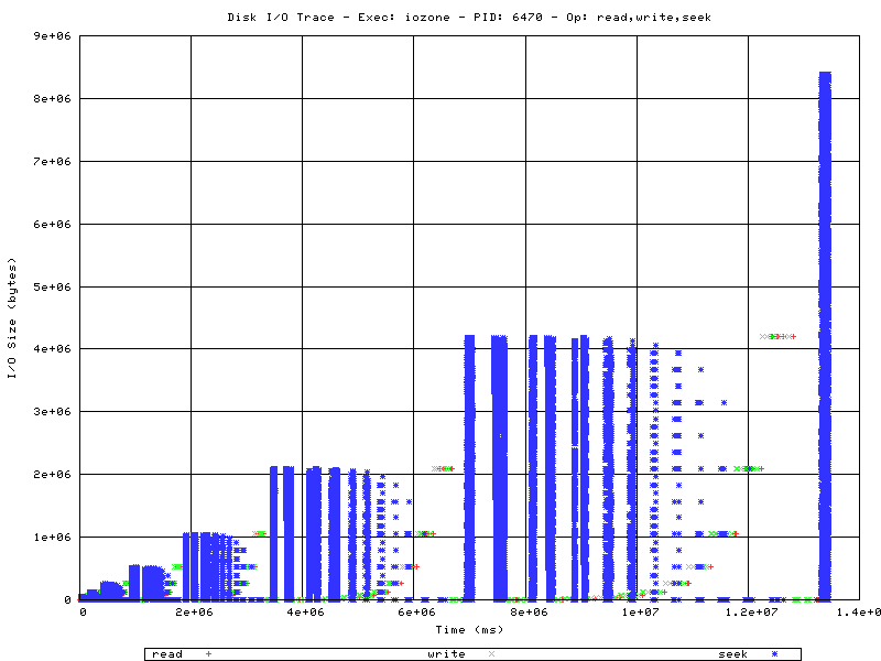
For traces that have many data points (e.g., traces that have over 50,000 events), the plot is broken up into subplots. In the example above, trace-disk-iozone-8974-read-3.plot.png is the 3rd graph for the iozone program and it plots read disk events.
An example graph that contains read, write and seek disk events would be trace-disk-iozone-6470-read,write,seek.plot.png and it looks like:
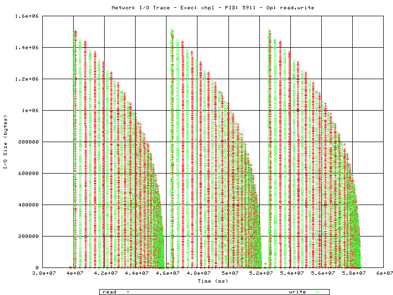
In addition to disk I/Os, all network reads and writes are also captured. To view the network I/O activity for a process, click on the file with the form 'trace-net-program-pid-op-graphnumber.plot.pdf'.
Here is an example plot from a Linpack process (xhpl):