Out-of-core classification of text documents

This is an example showing how scikit-learn can be used for classification using an out-of-core approach: learning from data that doesn’t fit into main memory. We make use of an online classifier, i.e., one that supports the partial_fit method, that will be fed with batches of examples. To guarantee that the features space remains the same over time we leverage a HashingVectorizer that will project each example into the same feature space. This is especially useful in the case of text classification where new features (words) may appear in each batch.

The dataset used in this example is Reuters-21578 as provided by the UCI ML repository. It will be automatically downloaded and uncompressed on first run.

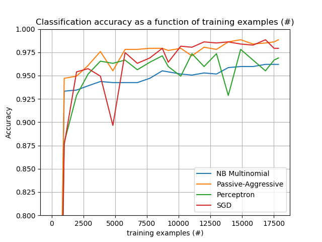
The plot represents the learning curve of the classifier: the evolution of classification accuracy over the course of the mini-batches. Accuracy is measured on the first 1000 samples, held out as a validation set.

To limit the memory consumption, we queue examples up to a fixed amount before feeding them to the learner.

# Authors: Eustache Diemert <[email protected]>
#          @FedericoV <https://github.com/FedericoV/>
# License: BSD 3 clause

from __future__ import print_function
from glob import glob
import itertools
import os.path
import re
import tarfile
import time
import sys

import numpy as np
import matplotlib.pyplot as plt
from matplotlib import rcParams

from sklearn.externals.six.moves import html_parser
from sklearn.externals.six.moves.urllib.request import urlretrieve
from sklearn.datasets import get_data_home
from sklearn.feature_extraction.text import HashingVectorizer
from sklearn.linear_model import SGDClassifier
from sklearn.linear_model import PassiveAggressiveClassifier
from sklearn.linear_model import Perceptron
from sklearn.naive_bayes import MultinomialNB


def _not_in_sphinx():
    # Hack to detect whether we are running by the sphinx builder
    return '__file__' in globals()

Reuters Dataset related routines

class ReutersParser(html_parser.HTMLParser):
    """Utility class to parse a SGML file and yield documents one at a time."""

    def __init__(self, encoding='latin-1'):
        html_parser.HTMLParser.__init__(self)
        self._reset()
        self.encoding = encoding

    def handle_starttag(self, tag, attrs):
        method = 'start_' + tag
        getattr(self, method, lambda x: None)(attrs)

    def handle_endtag(self, tag):
        method = 'end_' + tag
        getattr(self, method, lambda: None)()

    def _reset(self):
        self.in_title = 0
        self.in_body = 0
        self.in_topics = 0
        self.in_topic_d = 0
        self.title = ""
        self.body = ""
        self.topics = []
        self.topic_d = ""

    def parse(self, fd):
        self.docs = []
        for chunk in fd:
            self.feed(chunk.decode(self.encoding))
            for doc in self.docs:
                yield doc
            self.docs = []
        self.close()

    def handle_data(self, data):
        if self.in_body:
            self.body += data
        elif self.in_title:
            self.title += data
        elif self.in_topic_d:
            self.topic_d += data

    def start_reuters(self, attributes):
        pass

    def end_reuters(self):
        self.body = re.sub(r'\s+', r' ', self.body)
        self.docs.append({'title': self.title,
                          'body': self.body,
                          'topics': self.topics})
        self._reset()

    def start_title(self, attributes):
        self.in_title = 1

    def end_title(self):
        self.in_title = 0

    def start_body(self, attributes):
        self.in_body = 1

    def end_body(self):
        self.in_body = 0

    def start_topics(self, attributes):
        self.in_topics = 1

    def end_topics(self):
        self.in_topics = 0

    def start_d(self, attributes):
        self.in_topic_d = 1

    def end_d(self):
        self.in_topic_d = 0
        self.topics.append(self.topic_d)
        self.topic_d = ""


def stream_reuters_documents(data_path=None):
    """Iterate over documents of the Reuters dataset.

    The Reuters archive will automatically be downloaded and uncompressed if
    the `data_path` directory does not exist.

    Documents are represented as dictionaries with 'body' (str),
    'title' (str), 'topics' (list(str)) keys.

    """

    DOWNLOAD_URL = ('http://archive.ics.uci.edu/ml/machine-learning-databases/'
                    'reuters21578-mld/reuters21578.tar.gz')
    ARCHIVE_FILENAME = 'reuters21578.tar.gz'

    if data_path is None:
        data_path = os.path.join(get_data_home(), "reuters")
    if not os.path.exists(data_path):
        """Download the dataset."""
        print("downloading dataset (once and for all) into %s" %
              data_path)
        os.mkdir(data_path)

        def progress(blocknum, bs, size):
            total_sz_mb = '%.2f MB' % (size / 1e6)
            current_sz_mb = '%.2f MB' % ((blocknum * bs) / 1e6)
            if _not_in_sphinx():
                sys.stdout.write(
                    '\rdownloaded %s / %s' % (current_sz_mb, total_sz_mb))

        archive_path = os.path.join(data_path, ARCHIVE_FILENAME)
        urlretrieve(DOWNLOAD_URL, filename=archive_path,
                    reporthook=progress)
        if _not_in_sphinx():
            sys.stdout.write('\r')
        print("untarring Reuters dataset...")
        tarfile.open(archive_path, 'r:gz').extractall(data_path)
        print("done.")

    parser = ReutersParser()
    for filename in glob(os.path.join(data_path, "*.sgm")):
        for doc in parser.parse(open(filename, 'rb')):
            yield doc

Main

Create the vectorizer and limit the number of features to a reasonable maximum

vectorizer = HashingVectorizer(decode_error='ignore', n_features=2 ** 18,
                               alternate_sign=False)


# Iterator over parsed Reuters SGML files.
data_stream = stream_reuters_documents()

# We learn a binary classification between the "acq" class and all the others.
# "acq" was chosen as it is more or less evenly distributed in the Reuters
# files. For other datasets, one should take care of creating a test set with
# a realistic portion of positive instances.
all_classes = np.array([0, 1])
positive_class = 'acq'

# Here are some classifiers that support the `partial_fit` method
partial_fit_classifiers = {
    'SGD': SGDClassifier(max_iter=5),
    'Perceptron': Perceptron(tol=1e-3),
    'NB Multinomial': MultinomialNB(alpha=0.01),
    'Passive-Aggressive': PassiveAggressiveClassifier(tol=1e-3),
}


def get_minibatch(doc_iter, size, pos_class=positive_class):
    """Extract a minibatch of examples, return a tuple X_text, y.

    Note: size is before excluding invalid docs with no topics assigned.

    """
    data = [(u'{title}\n\n{body}'.format(**doc), pos_class in doc['topics'])
            for doc in itertools.islice(doc_iter, size)
            if doc['topics']]
    if not len(data):
        return np.asarray([], dtype=int), np.asarray([], dtype=int)
    X_text, y = zip(*data)
    return X_text, np.asarray(y, dtype=int)


def iter_minibatches(doc_iter, minibatch_size):
    """Generator of minibatches."""
    X_text, y = get_minibatch(doc_iter, minibatch_size)
    while len(X_text):
        yield X_text, y
        X_text, y = get_minibatch(doc_iter, minibatch_size)


# test data statistics
test_stats = {'n_test': 0, 'n_test_pos': 0}

# First we hold out a number of examples to estimate accuracy
n_test_documents = 1000
tick = time.time()
X_test_text, y_test = get_minibatch(data_stream, 1000)
parsing_time = time.time() - tick
tick = time.time()
X_test = vectorizer.transform(X_test_text)
vectorizing_time = time.time() - tick
test_stats['n_test'] += len(y_test)
test_stats['n_test_pos'] += sum(y_test)
print("Test set is %d documents (%d positive)" % (len(y_test), sum(y_test)))


def progress(cls_name, stats):
    """Report progress information, return a string."""
    duration = time.time() - stats['t0']
    s = "%20s classifier : \t" % cls_name
    s += "%(n_train)6d train docs (%(n_train_pos)6d positive) " % stats
    s += "%(n_test)6d test docs (%(n_test_pos)6d positive) " % test_stats
    s += "accuracy: %(accuracy).3f " % stats
    s += "in %.2fs (%5d docs/s)" % (duration, stats['n_train'] / duration)
    return s


cls_stats = {}

for cls_name in partial_fit_classifiers:
    stats = {'n_train': 0, 'n_train_pos': 0,
             'accuracy': 0.0, 'accuracy_history': [(0, 0)], 't0': time.time(),
             'runtime_history': [(0, 0)], 'total_fit_time': 0.0}
    cls_stats[cls_name] = stats

get_minibatch(data_stream, n_test_documents)
# Discard test set

# We will feed the classifier with mini-batches of 1000 documents; this means
# we have at most 1000 docs in memory at any time.  The smaller the document
# batch, the bigger the relative overhead of the partial fit methods.
minibatch_size = 1000

# Create the data_stream that parses Reuters SGML files and iterates on
# documents as a stream.
minibatch_iterators = iter_minibatches(data_stream, minibatch_size)
total_vect_time = 0.0

# Main loop : iterate on mini-batches of examples
for i, (X_train_text, y_train) in enumerate(minibatch_iterators):

    tick = time.time()
    X_train = vectorizer.transform(X_train_text)
    total_vect_time += time.time() - tick

    for cls_name, cls in partial_fit_classifiers.items():
        tick = time.time()
        # update estimator with examples in the current mini-batch
        cls.partial_fit(X_train, y_train, classes=all_classes)

        # accumulate test accuracy stats
        cls_stats[cls_name]['total_fit_time'] += time.time() - tick
        cls_stats[cls_name]['n_train'] += X_train.shape[0]
        cls_stats[cls_name]['n_train_pos'] += sum(y_train)
        tick = time.time()
        cls_stats[cls_name]['accuracy'] = cls.score(X_test, y_test)
        cls_stats[cls_name]['prediction_time'] = time.time() - tick
        acc_history = (cls_stats[cls_name]['accuracy'],
                       cls_stats[cls_name]['n_train'])
        cls_stats[cls_name]['accuracy_history'].append(acc_history)
        run_history = (cls_stats[cls_name]['accuracy'],
                       total_vect_time + cls_stats[cls_name]['total_fit_time'])
        cls_stats[cls_name]['runtime_history'].append(run_history)

        if i % 3 == 0:
            print(progress(cls_name, cls_stats[cls_name]))
    if i % 3 == 0:
        print('\n')

Out:

Test set is 870 documents (58 positive)
                 SGD classifier :          994 train docs (   121 positive)    870 test docs (    58 positive) accuracy: 0.876 in 0.88s ( 1128 docs/s)
          Perceptron classifier :          994 train docs (   121 positive)    870 test docs (    58 positive) accuracy: 0.878 in 0.98s ( 1013 docs/s)
      NB Multinomial classifier :          994 train docs (   121 positive)    870 test docs (    58 positive) accuracy: 0.933 in 0.99s ( 1005 docs/s)
  Passive-Aggressive classifier :          994 train docs (   121 positive)    870 test docs (    58 positive) accuracy: 0.947 in 0.99s ( 1002 docs/s)


                 SGD classifier :         3845 train docs (   554 positive)    870 test docs (    58 positive) accuracy: 0.949 in 2.88s ( 1332 docs/s)
          Perceptron classifier :         3845 train docs (   554 positive)    870 test docs (    58 positive) accuracy: 0.966 in 2.92s ( 1318 docs/s)
      NB Multinomial classifier :         3845 train docs (   554 positive)    870 test docs (    58 positive) accuracy: 0.944 in 2.98s ( 1288 docs/s)
  Passive-Aggressive classifier :         3845 train docs (   554 positive)    870 test docs (    58 positive) accuracy: 0.976 in 2.99s ( 1286 docs/s)


                 SGD classifier :         6755 train docs (   920 positive)    870 test docs (    58 positive) accuracy: 0.963 in 4.86s ( 1389 docs/s)
          Perceptron classifier :         6755 train docs (   920 positive)    870 test docs (    58 positive) accuracy: 0.956 in 4.86s ( 1389 docs/s)
      NB Multinomial classifier :         6755 train docs (   920 positive)    870 test docs (    58 positive) accuracy: 0.943 in 4.87s ( 1387 docs/s)
  Passive-Aggressive classifier :         6755 train docs (   920 positive)    870 test docs (    58 positive) accuracy: 0.978 in 4.87s ( 1386 docs/s)


                 SGD classifier :         9191 train docs (  1191 positive)    870 test docs (    58 positive) accuracy: 0.964 in 6.47s ( 1419 docs/s)
          Perceptron classifier :         9191 train docs (  1191 positive)    870 test docs (    58 positive) accuracy: 0.960 in 6.48s ( 1419 docs/s)
      NB Multinomial classifier :         9191 train docs (  1191 positive)    870 test docs (    58 positive) accuracy: 0.954 in 6.48s ( 1417 docs/s)
  Passive-Aggressive classifier :         9191 train docs (  1191 positive)    870 test docs (    58 positive) accuracy: 0.977 in 6.48s ( 1417 docs/s)


                 SGD classifier :        12010 train docs (  1551 positive)    870 test docs (    58 positive) accuracy: 0.986 in 8.34s ( 1440 docs/s)
          Perceptron classifier :        12010 train docs (  1551 positive)    870 test docs (    58 positive) accuracy: 0.960 in 8.34s ( 1440 docs/s)
      NB Multinomial classifier :        12010 train docs (  1551 positive)    870 test docs (    58 positive) accuracy: 0.953 in 8.35s ( 1438 docs/s)
  Passive-Aggressive classifier :        12010 train docs (  1551 positive)    870 test docs (    58 positive) accuracy: 0.980 in 8.35s ( 1438 docs/s)


                 SGD classifier :        14892 train docs (  1902 positive)    870 test docs (    58 positive) accuracy: 0.984 in 9.94s ( 1498 docs/s)
          Perceptron classifier :        14892 train docs (  1902 positive)    870 test docs (    58 positive) accuracy: 0.978 in 9.94s ( 1497 docs/s)
      NB Multinomial classifier :        14892 train docs (  1902 positive)    870 test docs (    58 positive) accuracy: 0.960 in 9.95s ( 1496 docs/s)
  Passive-Aggressive classifier :        14892 train docs (  1902 positive)    870 test docs (    58 positive) accuracy: 0.989 in 9.95s ( 1496 docs/s)


                 SGD classifier :        17524 train docs (  2246 positive)    870 test docs (    58 positive) accuracy: 0.979 in 11.71s ( 1495 docs/s)
          Perceptron classifier :        17524 train docs (  2246 positive)    870 test docs (    58 positive) accuracy: 0.967 in 11.72s ( 1495 docs/s)
      NB Multinomial classifier :        17524 train docs (  2246 positive)    870 test docs (    58 positive) accuracy: 0.962 in 11.72s ( 1494 docs/s)
  Passive-Aggressive classifier :        17524 train docs (  2246 positive)    870 test docs (    58 positive) accuracy: 0.986 in 11.73s ( 1494 docs/s)

Plot results

def plot_accuracy(x, y, x_legend):
    """Plot accuracy as a function of x."""
    x = np.array(x)
    y = np.array(y)
    plt.title('Classification accuracy as a function of %s' % x_legend)
    plt.xlabel('%s' % x_legend)
    plt.ylabel('Accuracy')
    plt.grid(True)
    plt.plot(x, y)


rcParams['legend.fontsize'] = 10
cls_names = list(sorted(cls_stats.keys()))

# Plot accuracy evolution
plt.figure()
for _, stats in sorted(cls_stats.items()):
    # Plot accuracy evolution with #examples
    accuracy, n_examples = zip(*stats['accuracy_history'])
    plot_accuracy(n_examples, accuracy, "training examples (#)")
    ax = plt.gca()
    ax.set_ylim((0.8, 1))
plt.legend(cls_names, loc='best')

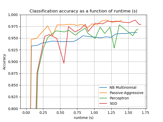
plt.figure()
for _, stats in sorted(cls_stats.items()):
    # Plot accuracy evolution with runtime
    accuracy, runtime = zip(*stats['runtime_history'])
    plot_accuracy(runtime, accuracy, 'runtime (s)')
    ax = plt.gca()
    ax.set_ylim((0.8, 1))
plt.legend(cls_names, loc='best')

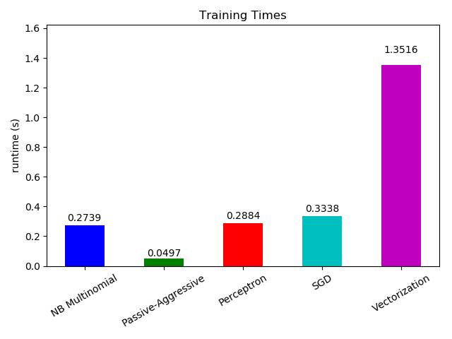
# Plot fitting times
plt.figure()
fig = plt.gcf()
cls_runtime = []
for cls_name, stats in sorted(cls_stats.items()):
    cls_runtime.append(stats['total_fit_time'])

cls_runtime.append(total_vect_time)
cls_names.append('Vectorization')
bar_colors = ['b', 'g', 'r', 'c', 'm', 'y']

ax = plt.subplot(111)
rectangles = plt.bar(range(len(cls_names)), cls_runtime, width=0.5,
                     color=bar_colors)

ax.set_xticks(np.linspace(0, len(cls_names) - 1, len(cls_names)))
ax.set_xticklabels(cls_names, fontsize=10)
ymax = max(cls_runtime) * 1.2
ax.set_ylim((0, ymax))
ax.set_ylabel('runtime (s)')
ax.set_title('Training Times')


def autolabel(rectangles):
    """attach some text vi autolabel on rectangles."""
    for rect in rectangles:
        height = rect.get_height()
        ax.text(rect.get_x() + rect.get_width() / 2.,
                1.05 * height, '%.4f' % height,
                ha='center', va='bottom')
        plt.setp(plt.xticks()[1], rotation=30)


autolabel(rectangles)
plt.tight_layout()
plt.show()

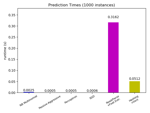
# Plot prediction times
plt.figure()
cls_runtime = []
cls_names = list(sorted(cls_stats.keys()))
for cls_name, stats in sorted(cls_stats.items()):
    cls_runtime.append(stats['prediction_time'])
cls_runtime.append(parsing_time)
cls_names.append('Read/Parse\n+Feat.Extr.')
cls_runtime.append(vectorizing_time)
cls_names.append('Hashing\n+Vect.')

ax = plt.subplot(111)
rectangles = plt.bar(range(len(cls_names)), cls_runtime, width=0.5,
                     color=bar_colors)

ax.set_xticks(np.linspace(0, len(cls_names) - 1, len(cls_names)))
ax.set_xticklabels(cls_names, fontsize=8)
plt.setp(plt.xticks()[1], rotation=30)
ymax = max(cls_runtime) * 1.2
ax.set_ylim((0, ymax))
ax.set_ylabel('runtime (s)')
ax.set_title('Prediction Times (%d instances)' % n_test_documents)
autolabel(rectangles)
plt.tight_layout()
plt.show()

• 
• 
• 
• 

Total running time of the script: ( 0 minutes 12.568 seconds)