m_circle

パラメータ

gain

ゲインベクトル (単位:DB). デフォルト値は

gain

=[-12 -8 -6 -5 -4 -3 -2 -1.4 -1 -.5 0.25 0.5 0.7 1 1.4 2 2.3 3 4 5 6 8 12]

説明

m_circle は,複素平面(Re,Im)に gain引数で指定した 等ゲイン等高線を描画します.

gainのデフォルト値は:

[-12 -8 -6 -5 -4 -3 -2 -1.4 -1 -.5 0.25 0.5 0.7 1 1.4 2 2.3 3 4 5 6 8 12]

m_circle は nyquistと共に使用されます.

この関数は,hallchart 関数で代替されます.

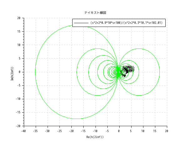
例

s=poly(0,'s')
h=syslin('c',(s^2+2*0.9*10*s+100)/(s^2+2*0.3*10.1*s+102.01))
nyquist(h,0.01,100,'(s^2+2*0.9*10*s+100)/(s^2+2*0.3*10.1*s+102.01)')
m_circle();

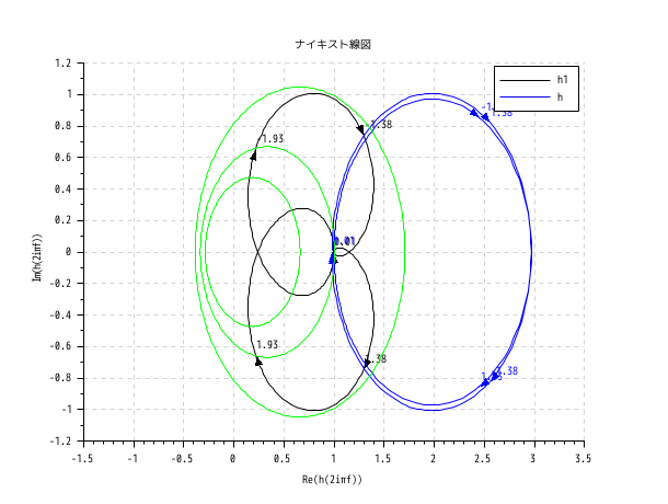
clf();
s=poly(0,'s')
h=syslin('c',(s^2+2*0.9*10*s+100)/(s^2+2*0.3*10.1*s+102.01))
h1=h*syslin('c',(s^2+2*0.1*15.1*s+228.01)/(s^2+2*0.9*15*s+225))
nyquist([h1;h],0.01,100,['h1';'h'])
m_circle([-8 -6 -4]);

参照

• nyquist — ナイキスト線図
• nicholschart — ニコルス線図
• black — Black図 (ニコルス線図)