- Ajuda do Scilab
- Biblioteca de Gráficos
- 2d_plot
- LineSpec
- Matplot
- Matplot1
- Matplot_properties
- Sfgrayplot
- Sgrayplot
- champ
- champ1
- champ_properties
- contour2d
- contour2di
- contourf
- errbar
- fchamp
- fec
- fgrayplot
- fplot2d
- grayplot
- grayplot_properties
- graypolarplot
- histplot
- paramfplot2d
- plot
- plot2d
- plot2d2
- plot2d3
- plot2d4
- polarplot
- comet
- contour2dm
- fec properties
- scatter
Sfgrayplot
esboço 2d suave de uma superfÃcie definida por uma função utilizando cores
Seqüência de Chamamento
Sfgrayplot(x,y,f,<opt_args>)
Sfgrayplot(x,y,f [,strf, rect, nax, zminmax, colminmax, mesh, colout])
Parâmetros
- x,y
vetores linhas de reais de tamanhos n1 e n2.
- f
função do Scilab (z=f(x,y))
- <opt_args>
representa uma seqüência de declarações
key1=value1,
                            key2=value2
,... ondekey1,key2,...podem ser um dos seguintes: strf, rect, nax, zminmax, colminmax, mesh, colout (ver plot2d para os três primeiros e fec para os quatro últimos).- strf,rect,nax
ver plot2d.
- zminmax, colminmax, mesh, colout
ver fec.
Descrição
Sfgrayplot é o mesmo que
fgrayplot mas o esboço é suavizado. A função
fec é utilizada para suavização. A superfÃcie é
esboçada assumindo-se que é linear em um conjunto de triângulos
construÃdos a partir do grid (aqui, com n1=5, n2=3):
_____________
| /| /| /| /|
|/_|/_|/_|/_|
| /| /| /| /|
|/_|/_|/_|/_|
A função colorbar pode ser utilizada para se visualizar a escala de cores (mas você deve saber (ou computar) os valores mÃnimo e máximo).
Ao invés de Sfgrayplot, você pode usar Sgrayplot este pode ser um pouco mais rápido.
Entre com o comando Sfgrayplot() para visualizar
uma demonstração.
Exemplos
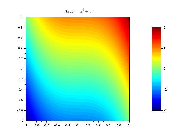
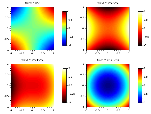
// exemplo #1: esboço de 4 superfÃcies function z=surf1(x, y), z=x*y, endfunction function z=surf2(x, y), z=x^2-y^2, endfunction function z=surf3(x, y), z=x^3+y^2, endfunction function z=surf4(x, y), z=x^2+y^2, endfunction clf() set(gcf(),"color_map",[jetcolormap(64);hotcolormap(64)]) x = linspace(-1,1,60); y = linspace(-1,1,60); drawlater(); subplot(2,2,1) colorbar(-1,1,[1,64]) Sfgrayplot(x,y,surf1,strf="041",colminmax=[1,64]) xtitle("f(x,y) = x*y") subplot(2,2,2) colorbar(-1,1,[65,128]) Sfgrayplot(x,y,surf2,strf="041",colminmax=[65,128]) xtitle("f(x,y) = x^2-y^2") subplot(2,2,3) colorbar(-1,2,[65,128]) Sfgrayplot(x,y,surf3,strf="041",colminmax=[65,128]) xtitle("f(x,y) = x^3+y^2") subplot(2,2,4) colorbar(0,2,[1,64]) Sfgrayplot(x,y,surf4,strf="041",colminmax=[1,64]) xtitle("f(x,y) = x^2+y^2") drawnow(); show_window()
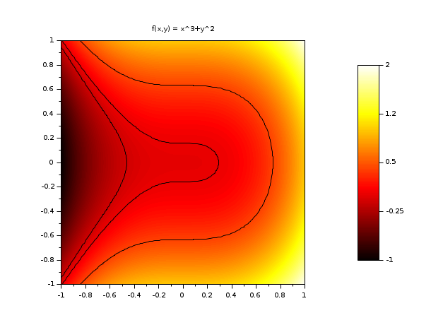
// exemplo #2: esboço de surf3 e adição de algumas linhas de contorno
function z=surf3(x, y), z=x^3+y^2, endfunction
clf()
x = linspace(-1,1,60);
y = linspace(-1,1,60);
set(gcf(),"color_map",hotcolormap(128))
drawlater();
colorbar(-1,2)
Sfgrayplot(x,y,surf3,strf="041")
contour2d(x,y,surf3,[-0.1, 0.025, 0.4],style=[1 1 1],strf="000")
xtitle("f(x,y) = x^3+y^2")
drawnow();
show_window()
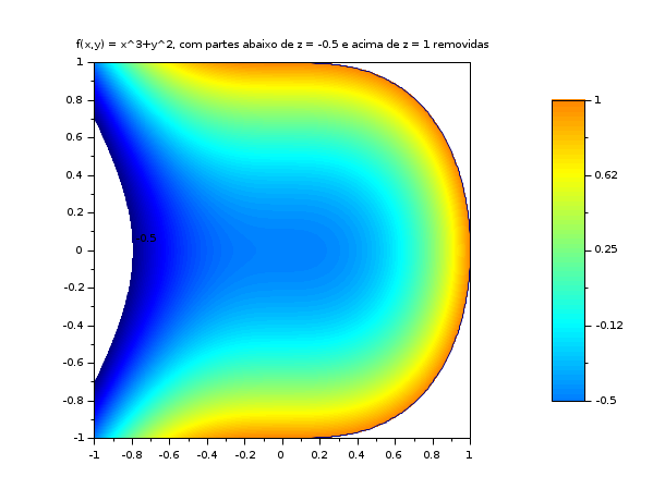
// exemplo #3: esboço de surf3 e uso dos argumentos opcionais zminmax e colout
//             para restringir o esboço em -0.5<= z <= 1
function z=surf3(x, y), z=x^3+y^2, endfunction
clf()
x = linspace(-1,1,60);
y = linspace(-1,1,60);
set(gcf(),"color_map",jetcolormap(128))
drawlater();
zminmax = [-0.5 1]; colors=[32 96];
colorbar(zminmax(1),zminmax(2),colors)
Sfgrayplot(x, y, surf3, strf="041", zminmax=zminmax, colout=[0 0], colminmax=colors)
contour2d(x,y,surf3,[-0.5, 1],style=[1 1 1],strf="000")
xtitle("f(x,y) = x^3+y^2, com partes abaixo de z = -0.5 e acima de z = 1 removidas")
drawnow();
show_window()
Comments
Add a comment:
Please login to comment this page.