sgrid
s-plane grid lines.
Syntax
sgrid()
sgrid(zeta,wn [,colors])
sgrid(['new',] zeta,wn [,colors])
sgrid(zeta,wn [,'new'] [,colors])
Arguments
- zeta
array of damping factors. Only values in
[0
                            1]
are taken into account. The default value is[0 0.16 0.34 0.5 0.64 0.76 0.86 0.94 0.985 1].- wn
array of natural frequencies in Hz. only positive values are taken into account. If not given it is computed by the program to fit with the boundaries of the plot.
- colors
a scalar or an 2 element array with integer values (color index).
Description
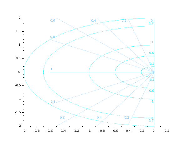
Plots selected curves of constant damping ratio (selection given
by zeta) and constant natural frequency
(selection given by wn).
The colors argument may be used to assign a
color for constant damping ratio curves
(colors(2)) and for constant natural
frequency curves (colors(1)).
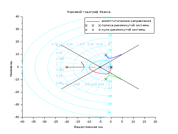
The sgrid function is often used to draw a grid
for evens root locus of continuous time linear systems. In such a
case the sgrid function should be called after
the call to evans. For discrete time linear
systems one should use zgrid function instead.
The optional argument 'new' can be used to
erase the graphic window before plotting the grid.
Comments
Add a comment:
Please login to comment this page.