IC2D: Interactive Control and Debugging of Distribution

IC2D is a graphical environment for remote monitoring and steering of distributed and grid applications . IC2D is built on top of ProActive that provides asynchronous calls and migration.

IC2D is available in the form of a Java standalone application based on Eclipse Rich Client Platform (RCP) , available for several platforms (Windows, Linux, Mac OSX,)

39.1. Monitoring and Control

IC2D is based on a plugin architecture and provides 2 plugins in relation to the monitoring and the control of ProActive applications:

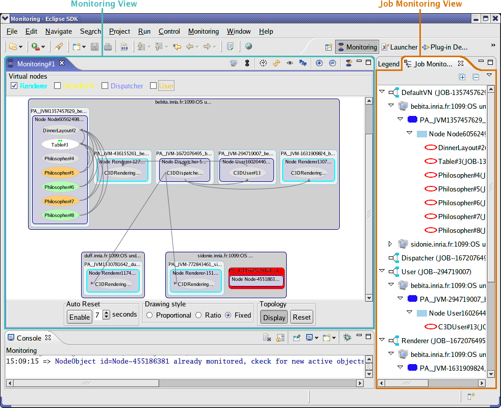
The Monitoring plugin which provides a graphical visualisation for hosts, Java Virtual Machines, and active objects, including the topology and the volume of communications
The Job Monitoring plugin which provides a tree representation of all these objects.

39.1.1. The Monitoring plugin

39.1.1.1. The Monitoring perspective

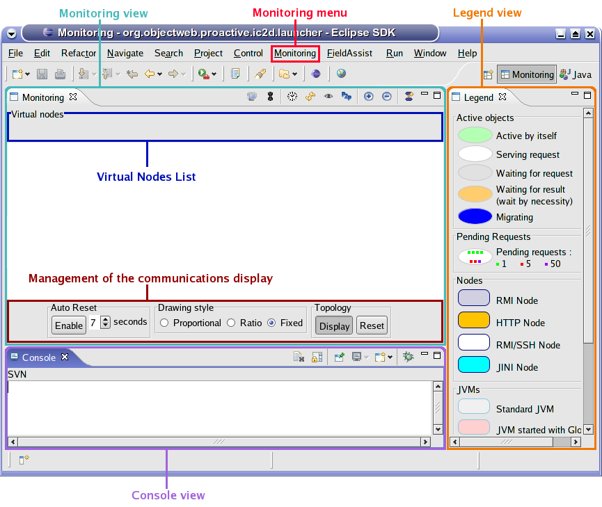
The Monitoring plugin provides the Monitoring perspective displayed in the Figure 39.1, “The Monitoring Perspective” .

This perspective defines the following set of views :

The Monitoring view: contains the graphical visualisation for ProActive objects
The Legend view: contains the legend corresponding to the Monitoring view's content
The Console view: contains log corresponding to the Monitoring view's events

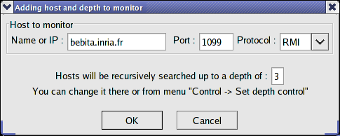
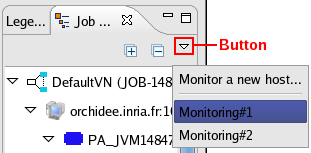
Figure 39.1. The Monitoring Perspective

39.1.1.2. Monitor a new host

In order to monitor a new host:

open the Monitoring Perspective: Window->Open Perspective->Other...->Monitoring (in the standalone IC2D, it should be already opened because it is the default perspective)
select Monitoring->Monitor a new host... , it opens the "Monitor a new Host" dialog displayed in the Figure 39.2, “Monitor New Host Dialog”
enter informations required about the host to monitor, and click OK

Figure 39.2. Monitor New Host Dialog

39.1.1.3. The Monitoring buttons

Here the buttons proposed in the monitoring view:

Figure 39.3. Monitor a new host

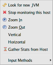
Display the "Monitor a new host" dialog in order to monitor a new host.

Figure 39.4. Set depth control

Display the "Set Depth Control" dialog in order to change the depth variable. For example: We have 3 hosts: 'A' 'B' and 'C'. And on A there is an active object 'aoA' which communicates with another active object 'aoB' which is on B. This one communicates with an active object 'aoC' on C, and aoA don't communicate with aoC. Then if we monitor A, and if the depth is 1, we will not see aoC.

Figure 39.5. Set time to refresh

Display the "Set Time to Refresh" dialog in order to change the time to refresh the model. And find the new added objects.

Figure 39.6. Refresh

Refreh the model.

Figure 39.7. Enable/Disable Monitoring

When the eye is opened the monitoring is activated.

Figure 39.8. Show P2P objects

Allows to see or not the P2P objects.

Figure 39.9. Zoom In

Figure 39.10. Zoom out

Figure 39.11. New Monitoring View

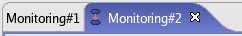
Open a new Monitoring view. This button can be used in any perspective. The new created view will be named 'Monitoring#number_of_this_view'

39.1.1.4. The Virtual Nodes list

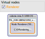
At the top of the Monitoring View, one can find the Virtual Nodes list . When some nodes are monirored, their virtual nodes are added to this list. And when a virtual node is checked, all its nodes are highlighted.

Figure 39.12. Virtual nodes List

39.1.1.5. Management of the communications display

At the bottom of the Monitoring view, one can find a set of buttons used to manage the communications display:

Auto Reset : Automatic reset of communications, you can specify the auto reset time
Display topology : show/hide communications
Proportional : arrows thickness is proportional to the number of requests
Ratio : arrows thickness uses a ratio of the number of requests
Fixed : arrows always have the same thickness whatever the number of communications
Topology : show/hide communications, and erase all communications
Monitoring enable : listen or not communications between active objects

39.1.1.6. Example

The Figure 39.16, “Monitoring of 2 applications” shows an example where 3 hosts are monitored. The applications running are philosophers and C3D ( Section 5.1, “C3D: A distributed 3D renderer” ).

39.1.2. The Job Monitoring plugin

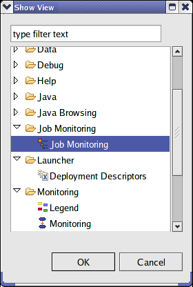
To look at the tree representation of the monitored objects, one have to open the Job Monitoring view .

For that, select Window->Show view->Other...->Job Monitoring->Job Monitoring .

Figure 39.13. Select the Job Monitoring view in the list

Then, select the model that you want to monitor. Each name corresponds to a monitoring view. You can also monitor a new host.

Figure 39.14. Select the Monitoring model

Figure 39.15. The monitoring views

One can see in the Figure 39.16, “Monitoring of 2 applications” an example of a tree representation of some monitored objects.

Figure 39.16. Monitoring of 2 applications

39.1.3. The TimIt plugin

The TimIt plugin for IC2D provides the ability to profile a distributed application in real time .

The activation of profiling is done through a TimItTechnicalService attached to the virtual node that contains active objects the user want to profile.

In your deployement descriptor you have to declare the technical service :

                        
             <technicalServices>
                 <technicalServiceDefinition id="profile" class=
"org.objectweb.proactive.benchmarks.timit.util.service.TimItTechnicalService">
                    <arg name="timitActivation" value="all"/>          
                    <arg name="reduceResults" value="false"/>
                    <arg name="printOutput" value="false"/>     
                 </technicalServiceDefinition>
             </technicalServices>

Then use the defined id in the virtualNode definition :

                        
            <virtualNodesDefinition>
              <virtualNode name="Workers" technicalServiceId="profile"/>
            </virtualNodesDefinition>

As shown in Figure 39.17, “ Gathering stats (right-click in Monitoring View). ” the user can collect some usefull information from active objects during the execution time to analyse the application performance .

Figure 39.17. Gathering stats (right-click in Monitoring View).

For that, 3 views are available.

39.1.3.1. TimIt Main View

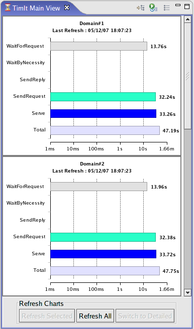
The main view shown in Figure 39.18, “ Time snapshots for 2 active objects ” is composed of bar charts (one chart per active object). Each chart represents cumulated times of different states that the active object has been in.

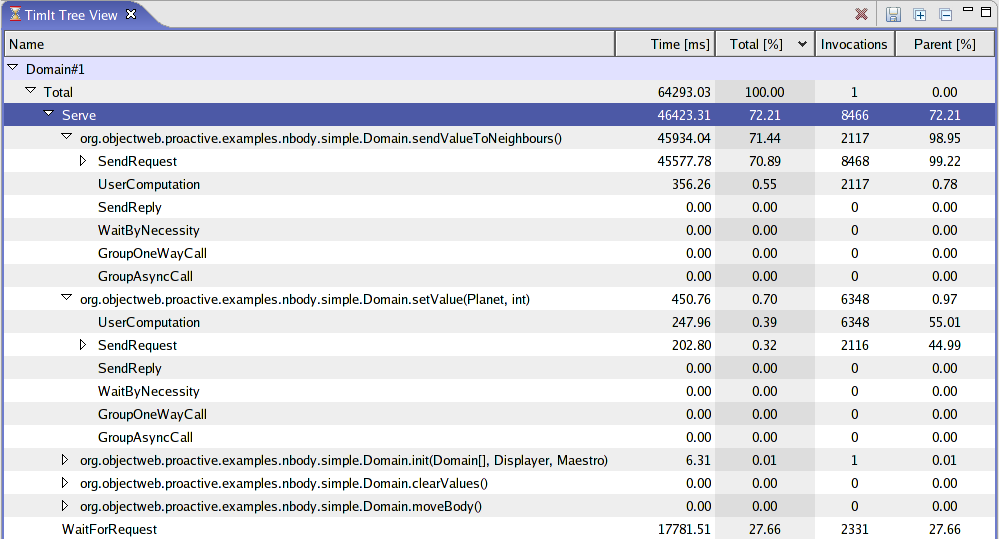
Figure 39.18. Time snapshots for 2 active objects

39.1.3.2. TimIt Tree View

The tree view shown in Figure 39.19, “ Hierarchical decomposition of the total time of an active object ” allows a more detailed hierarchical decomposition view of the total time for a particular active object.

Suppose that your active object class is :

	package org.objectweb.user.example;

	public class ActiveObjectClass{
		public ActiveObjectClass(){}

		public void methodA(Integer i, Double d){}

		private void methodB(){}

		protected void methodC(){}
	}

The hierarchical time decomposition includes times of user active object class methods (that must be public and non-final) served as requests (ie called by other active objects).

Total The total time since the creation of the active object.
- WaitForRequest The time spent on waiting for requests.
- Serve The time spent on serving incoming requests.
  - org.objectweb.user.example.ActiveObjectClass.methodA(Integer, Double) The time spent on serving the methodA as a request (local calls to this method are not included).
    
    UserComputation The time spent on computation (ie everything except communications).
    
    SendRequest The time spent on sending requests to other active objects.
    
    BeforeSerialization The time spent before the serialization of requests to other active objects.
    
    Serialization The time spent on serializing requests to other active objects.
    
    AfterSerialization The time spent after the serialization af requests to other active objects.
    
    LocalCopy The time spent on copying arguments in case of communications with local active objects.
    
    SendReply The time spent on sending replies to other active objects.
    
    GroupOneWayCall The time spent on performing asynchronous one way calls to groups of active objects (void methods).
    
    GroupAsyncCall The time spent on performing asynchronous calls to groups of active objects (non-void methods).
    
    WaitByNecessity The time spent on waiting by necessity.

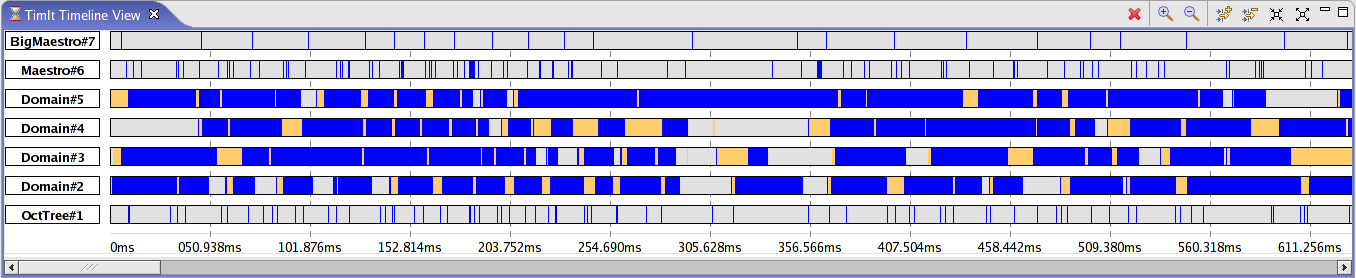
Figure 39.19. Hierarchical decomposition of the total time of an active object

39.1.3.3. TimIt Timeline View

The timeline view shown in Figure 39.20, “ The timeline for 7 active objects ” represents all events that were recorded during a certain time-lapse. The color of each event correspond to colors defined in the Legend view. This view shows the intensity of particular states (serving, waiting for request, etc...).

Figure 39.20. The timeline for 7 active objects

39.2. Launcher

39.2.1. Principles

The launcher allows users to launch applications directly from an XML descriptor file, without any script. The new XML descriptor is nearly the same as classical descriptor files, the syntax is only extended. The deployment will be done in two different phasis.

first, a new node, a "main node" will be created and activated and then, it is this node that will deploy the rest of the application.

39.2.2. MainDefinition tag

A new tag has been introduced, just before the component definition tag. This tag is named "mainDefinition" and its syntax is:

        &lt;mainDefinition id="mainID"
        class="theClassToLaunchContainingAMainMethod"&gt;
        &lt;arg value="param1"&gt; &lt;arg value="param2"&gt;
        &lt;mapToVirtualNode value="main-Node"/&gt;
        &lt;/mainDefinition&gt;

Eventually, several mains might be defined so the id allows to identify all mainDefinitions.

The class attribute is the path where can be found the class to launch.

This class MUST contain a main method.

Then any number of parameters can be declared in arg tags. The parameters will be given to the main method in the same order the were declared.

And finally a mapToVirtualNode tag will link the main info to virtual node, declared with the same name in the virtualNodeDefinitions tag (in componentDefinition).

<?xml version="1.0" encoding="UTF-8"?>
<ProActiveDescriptor
    xmlns:xsi="http://www.w3.org/2001/XMLSchema-instance"
   
 xsi:noNamespaceSchemaLocation="http://www-sop.inria.fr/oasis/proactive/schema/DescriptorSchema.xsd"
>
    <!-- <security
        file="../../descriptors/c3dPolicy.xml"></security>
    -->
    <componentDefinition>
        <virtualNodesDefinition>
            <virtualNode name="Dispatcher" property="unique_singleAO" />
            <virtualNode name="Renderer" />
        </virtualNodesDefinition>
    </componentDefinition>
    <deployment>
        <register virtualNode="Dispatcher" />
        <mapping>
            <map virtualNode="Dispatcher">
                <jvmSet>
                    <currentJVM />
                </jvmSet>
            </map>
            <map virtualNode="Renderer">
                <jvmSet>
                    <vmName value="Jvm1" />
                    <vmName value="Jvm2" />
                    <vmName value="Jvm3" />
                    <vmName value="Jvm4" />
                </jvmSet>
            </map>
        </mapping>
        <jvms>
            <jvm name="Jvm1">
                <creation>
                    <processReference refid="localJVM" />
                </creation>
            </jvm>
            <jvm name="Jvm2">
                <creation>
                    <processReference refid="localJVM" />
                </creation>
            </jvm>
            <jvm name="Jvm3">
                <creation>
                    <processReference refid="localJVM" />
                </creation>
            </jvm>
            <jvm name="Jvm4">
                <creation>
                    <processReference refid="localJVM" />
                </creation>
            </jvm>
        </jvms>
    </deployment>
    <infrastructure>
        <processes>
            <processDefinition id="localJVM">
                <jvmProcess
                    class="org.objectweb.proactive.core.process.JVMNodeProcess">
                </jvmProcess>
            </processDefinition>
        </processes>
    </infrastructure>
</ProActiveDescriptor>

39.2.3. API

The Launcher class is located in the package org.objectweb.proactive.core.descriptor . To use it you will have to create a new instance of the launcher with the path of the XML descriptor (this descriptor must contain a mainDefinition tag ). The constructor will parse the file and reify a ProActiveDescriptor. You only have to call the activate() method on the launcher instance to launch the application.

For example:

Launcher launcher = new Launcher ("myDescriptor.xml") ;

launcher.activate() ;

you can also get the ProActiveDescriptor built by the launcher by calling the getDescriptor() method on the launcher instance.

ProActiveDescriptor pad = launcher.getDescriptor() ;

39.2.4. The Launcher Plug-in

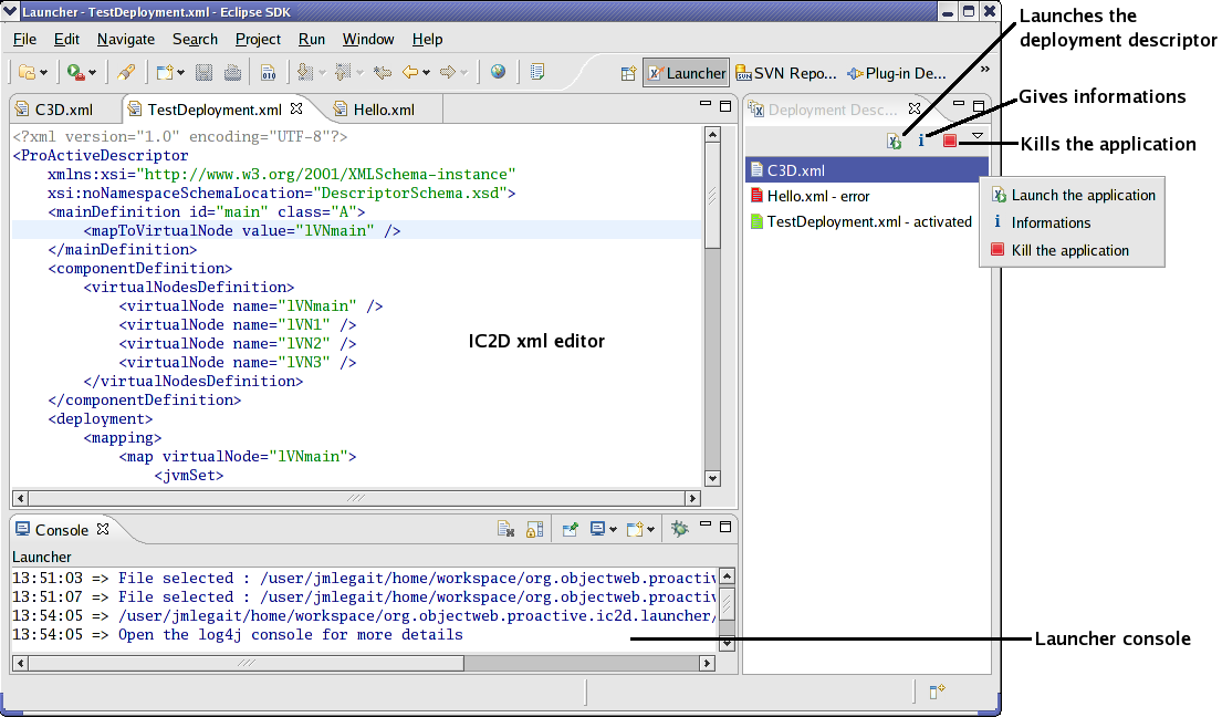
In order to launch a deployment descriptor , you must open your file with the IC2D XML Editor .

To use this editor, you have two possibilities:

39.2.4.1. First possibility

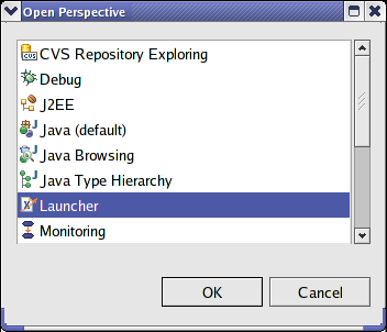
Open the Launcher perspective . Select: Window > Open perspective > Other... > Launcher

Figure 39.21. The "Open Perspective" window

Then select: File > Open File... and open your deployment descriptor, it will be opened with the IC2D XML editor. And its name will appear in the Deployment descriptors list.

39.2.4.2. Second possibility

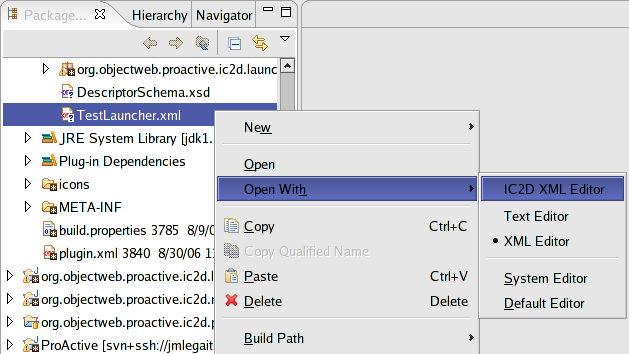
In the Navigator view, or another similar, a right click on the XML file allows you to open your file with the IC2D XML editor .

Figure 39.22. The open with action

39.2.4.3. The Launcher perspective

The Figure 39.23, “The Launcher perspective” represents the Launcher perspective containing an XML editor , a console , and the list of deployment descriptors .

To launch an application, select your file in the deployment descriptors list, and click on the launch icon.

You can kill the applications launched from a popup-menu in the "Deployment descriptors" list.

To see your application running, open the "Monitoring perspective" and monitor the corresponding host.

Figure 39.23. The Launcher perspective

39.3. Programming Tools

39.3.1. ProActive Wizards

These wizards will guide developpers to make complex operations with ProActive, such as installation, integration, configuration, or execution :

a ProActive installation wizard
a wizard that create applications using ProActive
an active object creation wizard
a configuration and execution wizard

Figure 39.24. A wizard popup

39.3.2. The ProActive Editor

This editor checks coding rules. It informs the developper of error concerning ProActive in his classes and can resolve some of these errors.

Figure 39.25. The editor error highlighting

39.4. The Guided Tour as Plugin

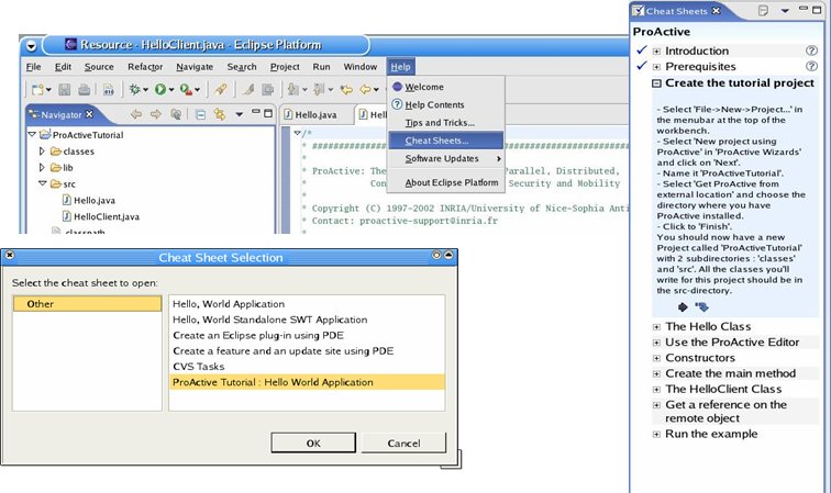
The aim of the guided tour is to provide a step by step explanation to the ProActive beginners.

Figure 39.26. The plugin's interface

This guided tour (that is actually eclipse cheat sheet) purposes:

To Explain ProActive to beginners
To make interactions with the user with simple situations
To Show the important points

Prev	Up	Next
Part VIII. Graphical User Interface (GUI) and tools	Table of Contents	Chapter 40. Interface with Matlab/Scilab